The Metastable Solitude
dated research updates
- date:
- updated:
- reading:
- 16 min
- authors:
- Bryan Gass, Madhurima Roy
contents (7)
- TL;DR
- Dated research updates
- 27 September 2026 — Nuclear sensitivity survives, but inheritance is filtered
- 1 October 2026 — Nuclear survival depends on boundaries and passage
- 3 October 2026 — The parts do not yet describe one altered star
- 5 October 2026 — Which parts of the hypothesis are now constrained?
- 8 October 2026 — Numerical reviews expose limits on the proposed histories
TL;DR
These are the dated updates on the Metastable Solitude research, from 27 September to 8 October 2026, moved here from the essay.
Dated research updates
The original hypothesis needs more than the fact that chemistry has timescales. Its stronger claim is that a physically realizable change of field background could disrupt the compatibility of those timescales, or alter the material supply needed for organized chemistry. The cosmological extension adds two further claims: arrival into and departure from suitable states could make sufficiently long histories rare, and that rarity could help explain the absence of detectable neighbors. The calculations below test different links in that argument; success at one link cannot establish the others.
27 September 2026 — Nuclear sensitivity survives, but inheritance is filtered
A changed core is a real response in the tested star
The stellar comparison starts from an ordinary hydrogen-exhausted model of a 15-solar-mass star with metallicity , then changes the specified nuclear rates before helium ignition. Opacity, the equation of state and the other microphysics remain ordinary. The star is allowed to adjust its temperature and structure. At helium exhaustion, the results are:
| Nuclear-rate scenario | Central carbon mass fraction | Carbon retained in the star, | Total carbon lost in winds, |
|---|---|---|---|
| Ordinary rates | 0.3742 | 0.7148 | 0.004064 |
| Hoyle energy +39.9 keV | 0.00217 | 0.1604 | 0.004020 |
| Hoyle energy −39.9 keV | 0.7487 | 1.3404 | 0.003903 |
| Correlated alpha change +200 ppm | 0.4130 | 0.7745 | 0.004050 |
The last row uses a much smaller Hoyle shift, +0.798 keV, together with a modeled carbon-capture response and an assumed ground-state channel fraction of one-half. It is not another version of the isolated +39.9-keV intervention. A finer ordinary stellar calculation gives central carbon near 0.378, so the large imposed-shift responses cannot be explained by that particular numerical refinement.1
This supports the nuclear-to-star link: thermal feedback does not necessarily erase a nuclear-rate change. It does not establish an altered field state, because the imposed rates have not been accompanied by all the other changes that the same field would cause.
The material that escapes carries a much smaller difference
In the +39.9-keV case, central carbon falls by about 99.4%, retained carbon by 77.6%, and total carbon lost in winds by only 1.1%. These are three different quantities. The wind largely samples material outside the altered core, and its total carbon includes carbon present initially; it is not the net amount of newly synthesized carbon delivered to another world.
Following the winds through the tested four-cohort enrichment histories leaves a gas C/O difference of about – dex. Ordinary wind and mixing alternatives can produce larger differences. Terminal explosions and remnants are absent from these calculations.1
For the inheritance hypothesis, the large core effect therefore establishes an upstream sensitivity, while the small wind effect weakens this particular route to a distinctive inherited signature. Neither result determines a planet's composition. The consequential comparison is the released, mixed, multi-element inventory from one consistent physical model, with ordinary mass loss and explosion alternatives included. A carbon-poor core alone cannot establish a carbon-poor world, still less a sterile one.
An energy shift does not yet establish a lost chemical capability
The molecular calculations test a different link. In the leading nonrelativistic Coulomb problem, rescaling the molecular geometry along with the characteristic length and energy recovers the same dimensionless electronic problem for the hydrogen and water examples. An energy barrier changing in electronvolts can therefore reflect a change of scale. It need not show that the relative timing of useful reactions and destructive reactions has become incompatible.
A separate driven three-state maintenance model retains a stationary “functional” population of about 99.43–99.65% as its imposed energy-scale parameter moves from 0.95 to 1.05. Its selected temperature, catalyst strength and dimensionless driving are the same throughout that scan. This is not a numerical demonstration of temperature adjustment rescuing function. Moreover, its cycle current changes by a factor of about 20.4 across the range: a highly occupied functional state does not by itself establish adequate throughput.2
These results challenge the shortcut from “molecular energies change” to “organized chemistry becomes impossible.” They do not show that real organisms adapt to another field background. A stronger test must define what the network has to accomplish—turnover, repair, information retention and energy supply—and ask whether those requirements can still be met across physically allowed environments under the same correlated change of molecular parameters. No narrow, universal chemical viability window has been established by these examples.
The field must actually reach the burning material
The screened stellar profile supplies a concrete failure of a proposed connection. Although the exterior field differs from its dense-Earth value, the region supplying 99% of the modeled nuclear luminosity has the same sampled electromagnetic coupling as dense Earth. Within this benchmark, screening removes the nuclear-rate contrast that was supposed to change the star.3
Consequently, the altered-rate stellar tracks above cannot simply be attached to this screened background. The former establish sensitivity to an imposed input; the latter fails to provide that input where burning occurs. This rejects the intended mechanism for this profile and coupling, rather than every possible field model. A successful replacement has to sustain the contrast inside the relevant matter while also satisfying its local force and energy constraints.
1 October 2026 — Nuclear survival depends on boundaries and passage
The nuclear extension asks whether a field history could change the inventory available before molecules or stars form. Three conditions must be separated: a nucleus can be bound, able to survive weak decay, and accessible through a production reaction. None follows automatically from either of the others.
For example, with the other particle masses fixed, deuteron binding between about 0.782 and 1.804 MeV closes the displayed deuteron beta-breakup while leaving ordinary pp fusion endothermic. The tested correlated local light-quark response instead leaves the binding at roughly 2.10–2.34 MeV, the dineutron unbound and pp fusion exothermic. This response envelope is a stipulated local sensitivity calculation, not an observational confidence region. Recovering the ordinary Reid93 binding to about 10 eV checks the baseline energy convention; it does not extend that local response into a finite alternative field theory.4
The distinction changes the inference: adjustable nuclear forces can cross these boundaries, but the tested field response does not. That is evidence against claiming a crossing in this model and range, not evidence that every field model is forbidden from crossing. Even a genuine pp threshold crossing would require recalculating the remaining production routes and the thermal reaction rates before concluding that stars cannot burn.
Time-dependent calculations test the history part more directly. In the prescribed Bonn B cycle, the tensor multiplier falls from 1 to 0.4, passes through an unbound regime, and returns to 1. With the same intermediate hold, increasing the ramp timescale from 0.02 to 0.2 to 2 in units of leaves returned bound fractions of approximately 0.23, 0.20 and 0.11. Returning to the original Hamiltonian does not return the nucleus to its original state.
Returned deuteron binding depends on the prescribed passage through a changing interaction, even after the original interaction is restored.
- t
- 1.4000 ħ/MeV = 9.21e−22 s
- tensor multiplier
- 1.000
- overlap with the original deuteron
- 0.2009
- Change in nuclear energy
- 4.2703 MeV
- Work by prescribed interaction
- 4.2703 MeV
data
Bonn B follows a prescribed smooth excursion from tensor multiplier 1 to 0.4 and back, holding for ℏ/MeV between ramps. The minimum lies below its verified infinite-volume binding threshold. The complete S/D Hamiltonian and its quadrature continuum are propagated, with time, momentum-grid, sudden-limit and independent ODE controls. Nuclear energy change is checked against the supplied work. The final projector measures returned binding; intermediate overlap with the original deuteron is not an instantaneous bound fraction. Passage times are diagnostic, not derived from a viable field. No irreversibility, hysteresis or thermal capture rate is claimed. The bound-to-bound scan is a separate Gaussian model ending at binding 0.3 MeV; it is not the Bonn B excursion.
| series | time | tensor multiplier | overlap or P(bound) | Change in nuclear energy [MeV] | Work by prescribed interaction [MeV] |
|---|---|---|---|---|---|
| cycle t [ħ/MeV] | 0.0005 | 1.000 | 1.0000 | 0.0001 | 0.0001 |
| cycle t [ħ/MeV] | 0.0020 | 1.000 | 1.0000 | 0.0020 | 0.0020 |
| cycle t [ħ/MeV] | 0.0035 | 0.999 | 1.0000 | 0.0060 | 0.0060 |
| cycle t [ħ/MeV] | 0.0050 | 0.999 | 1.0000 | 0.0121 | 0.0121 |
| cycle t [ħ/MeV] | 0.0065 | 0.998 | 1.0000 | 0.0203 | 0.0203 |
| cycle t [ħ/MeV] | 0.0080 | 0.997 | 1.0000 | 0.0306 | 0.0306 |
| cycle t [ħ/MeV] | 0.0095 | 0.996 | 1.0000 | 0.0430 | 0.0430 |
| cycle t [ħ/MeV] | 0.0110 | 0.995 | 1.0000 | 0.0573 | 0.0573 |
| cycle t [ħ/MeV] | 0.0125 | 0.993 | 1.0000 | 0.0736 | 0.0736 |
| cycle t [ħ/MeV] | 0.0140 | 0.992 | 1.0000 | 0.0918 | 0.0918 |
| cycle t [ħ/MeV] | 0.0155 | 0.990 | 1.0000 | 0.1119 | 0.1119 |
| cycle t [ħ/MeV] | 0.0170 | 0.988 | 1.0000 | 0.1338 | 0.1338 |
| cycle t [ħ/MeV] | 0.0185 | 0.986 | 1.0000 | 0.1576 | 0.1576 |
| cycle t [ħ/MeV] | 0.0200 | 0.983 | 1.0000 | 0.1831 | 0.1831 |
| cycle t [ħ/MeV] | 0.0215 | 0.981 | 1.0000 | 0.2104 | 0.2104 |
| cycle t [ħ/MeV] | 0.0230 | 0.978 | 1.0000 | 0.2393 | 0.2393 |
| cycle t [ħ/MeV] | 0.0245 | 0.975 | 1.0000 | 0.2699 | 0.2699 |
| cycle t [ħ/MeV] | 0.0260 | 0.972 | 1.0000 | 0.3021 | 0.3021 |
| cycle t [ħ/MeV] | 0.0275 | 0.969 | 1.0000 | 0.3358 | 0.3358 |
| cycle t [ħ/MeV] | 0.0290 | 0.966 | 1.0000 | 0.3710 | 0.3710 |
| cycle t [ħ/MeV] | 0.0305 | 0.962 | 1.0000 | 0.4077 | 0.4077 |
| cycle t [ħ/MeV] | 0.0320 | 0.959 | 0.9999 | 0.4459 | 0.4459 |
| cycle t [ħ/MeV] | 0.0335 | 0.955 | 0.9999 | 0.4854 | 0.4854 |
| cycle t [ħ/MeV] | 0.0350 | 0.951 | 0.9999 | 0.5262 | 0.5262 |
| cycle t [ħ/MeV] | 0.0365 | 0.947 | 0.9999 | 0.5684 | 0.5684 |
| cycle t [ħ/MeV] | 0.0380 | 0.943 | 0.9999 | 0.6117 | 0.6117 |
| cycle t [ħ/MeV] | 0.0395 | 0.939 | 0.9998 | 0.6563 | 0.6563 |
| cycle t [ħ/MeV] | 0.0410 | 0.935 | 0.9998 | 0.7020 | 0.7020 |
| cycle t [ħ/MeV] | 0.0425 | 0.930 | 0.9998 | 0.7488 | 0.7488 |
| cycle t [ħ/MeV] | 0.0440 | 0.926 | 0.9997 | 0.7966 | 0.7966 |
| cycle t [ħ/MeV] | 0.0455 | 0.921 | 0.9997 | 0.8455 | 0.8455 |
| cycle t [ħ/MeV] | 0.0470 | 0.916 | 0.9996 | 0.8952 | 0.8952 |
| cycle t [ħ/MeV] | 0.0485 | 0.911 | 0.9995 | 0.9459 | 0.9459 |
| cycle t [ħ/MeV] | 0.0500 | 0.906 | 0.9995 | 0.9974 | 0.9974 |
| cycle t [ħ/MeV] | 0.0515 | 0.901 | 0.9994 | 1.0498 | 1.0498 |
| cycle t [ħ/MeV] | 0.0530 | 0.896 | 0.9993 | 1.1028 | 1.1028 |
| cycle t [ħ/MeV] | 0.0545 | 0.891 | 0.9992 | 1.1566 | 1.1566 |
| cycle t [ħ/MeV] | 0.0560 | 0.885 | 0.9991 | 1.2110 | 1.2110 |
| cycle t [ħ/MeV] | 0.0575 | 0.880 | 0.9989 | 1.2661 | 1.2661 |
| cycle t [ħ/MeV] | 0.0590 | 0.874 | 0.9988 | 1.3216 | 1.3216 |
| cycle t [ħ/MeV] | 0.0605 | 0.869 | 0.9987 | 1.3777 | 1.3777 |
| cycle t [ħ/MeV] | 0.0620 | 0.863 | 0.9985 | 1.4342 | 1.4342 |
| cycle t [ħ/MeV] | 0.0635 | 0.857 | 0.9983 | 1.4911 | 1.4911 |
| cycle t [ħ/MeV] | 0.0650 | 0.851 | 0.9981 | 1.5484 | 1.5484 |
| cycle t [ħ/MeV] | 0.0665 | 0.845 | 0.9979 | 1.6060 | 1.6060 |
| cycle t [ħ/MeV] | 0.0680 | 0.839 | 0.9976 | 1.6639 | 1.6639 |
| cycle t [ħ/MeV] | 0.0695 | 0.833 | 0.9974 | 1.7219 | 1.7219 |
| cycle t [ħ/MeV] | 0.0710 | 0.827 | 0.9971 | 1.7801 | 1.7801 |
| cycle t [ħ/MeV] | 0.0725 | 0.821 | 0.9968 | 1.8385 | 1.8385 |
| cycle t [ħ/MeV] | 0.0740 | 0.814 | 0.9965 | 1.8969 | 1.8969 |
| cycle t [ħ/MeV] | 0.0755 | 0.808 | 0.9961 | 1.9554 | 1.9554 |
| cycle t [ħ/MeV] | 0.0770 | 0.802 | 0.9958 | 2.0138 | 2.0138 |
| cycle t [ħ/MeV] | 0.0785 | 0.795 | 0.9954 | 2.0722 | 2.0722 |
| cycle t [ħ/MeV] | 0.0800 | 0.789 | 0.9950 | 2.1304 | 2.1304 |
| cycle t [ħ/MeV] | 0.0815 | 0.782 | 0.9945 | 2.1886 | 2.1886 |
| cycle t [ħ/MeV] | 0.0830 | 0.776 | 0.9940 | 2.2465 | 2.2465 |
| cycle t [ħ/MeV] | 0.0845 | 0.769 | 0.9935 | 2.3042 | 2.3042 |
| cycle t [ħ/MeV] | 0.0860 | 0.763 | 0.9930 | 2.3617 | 2.3617 |
| cycle t [ħ/MeV] | 0.0875 | 0.756 | 0.9924 | 2.4188 | 2.4188 |
| cycle t [ħ/MeV] | 0.0890 | 0.749 | 0.9918 | 2.4756 | 2.4756 |
| cycle t [ħ/MeV] | 0.0905 | 0.743 | 0.9912 | 2.5321 | 2.5321 |
| cycle t [ħ/MeV] | 0.0920 | 0.736 | 0.9906 | 2.5881 | 2.5881 |
| cycle t [ħ/MeV] | 0.0935 | 0.729 | 0.9899 | 2.6437 | 2.6437 |
| cycle t [ħ/MeV] | 0.0950 | 0.722 | 0.9891 | 2.6988 | 2.6988 |
| cycle t [ħ/MeV] | 0.0965 | 0.716 | 0.9884 | 2.7534 | 2.7534 |
| cycle t [ħ/MeV] | 0.0980 | 0.709 | 0.9876 | 2.8074 | 2.8074 |
| cycle t [ħ/MeV] | 0.0995 | 0.702 | 0.9867 | 2.8609 | 2.8609 |
| cycle t [ħ/MeV] | 0.1010 | 0.696 | 0.9858 | 2.9138 | 2.9138 |
| cycle t [ħ/MeV] | 0.1025 | 0.689 | 0.9849 | 2.9660 | 2.9660 |
| cycle t [ħ/MeV] | 0.1040 | 0.682 | 0.9840 | 3.0176 | 3.0176 |
| cycle t [ħ/MeV] | 0.1055 | 0.675 | 0.9830 | 3.0685 | 3.0685 |
| cycle t [ħ/MeV] | 0.1070 | 0.669 | 0.9819 | 3.1188 | 3.1188 |
| cycle t [ħ/MeV] | 0.1085 | 0.662 | 0.9809 | 3.1683 | 3.1683 |
| cycle t [ħ/MeV] | 0.1100 | 0.655 | 0.9797 | 3.2170 | 3.2170 |
| cycle t [ħ/MeV] | 0.1115 | 0.648 | 0.9786 | 3.2650 | 3.2650 |
| cycle t [ħ/MeV] | 0.1130 | 0.642 | 0.9774 | 3.3122 | 3.3122 |
| cycle t [ħ/MeV] | 0.1145 | 0.635 | 0.9761 | 3.3586 | 3.3586 |
| cycle t [ħ/MeV] | 0.1160 | 0.629 | 0.9749 | 3.4042 | 3.4042 |
| cycle t [ħ/MeV] | 0.1175 | 0.622 | 0.9735 | 3.4489 | 3.4489 |
| cycle t [ħ/MeV] | 0.1190 | 0.616 | 0.9722 | 3.4928 | 3.4928 |
| cycle t [ħ/MeV] | 0.1205 | 0.609 | 0.9708 | 3.5359 | 3.5359 |
| cycle t [ħ/MeV] | 0.1220 | 0.603 | 0.9693 | 3.5780 | 3.5780 |
| cycle t [ħ/MeV] | 0.1235 | 0.596 | 0.9678 | 3.6193 | 3.6193 |
| cycle t [ħ/MeV] | 0.1250 | 0.590 | 0.9663 | 3.6597 | 3.6597 |
| cycle t [ħ/MeV] | 0.1265 | 0.584 | 0.9647 | 3.6992 | 3.6992 |
| cycle t [ħ/MeV] | 0.1280 | 0.577 | 0.9631 | 3.7378 | 3.7378 |
| cycle t [ħ/MeV] | 0.1295 | 0.571 | 0.9615 | 3.7755 | 3.7755 |
| cycle t [ħ/MeV] | 0.1310 | 0.565 | 0.9598 | 3.8122 | 3.8122 |
| cycle t [ħ/MeV] | 0.1325 | 0.559 | 0.9581 | 3.8481 | 3.8481 |
| cycle t [ħ/MeV] | 0.1340 | 0.553 | 0.9563 | 3.8830 | 3.8830 |
| cycle t [ħ/MeV] | 0.1355 | 0.547 | 0.9545 | 3.9170 | 3.9170 |
| cycle t [ħ/MeV] | 0.1370 | 0.541 | 0.9526 | 3.9501 | 3.9501 |
| cycle t [ħ/MeV] | 0.1385 | 0.535 | 0.9508 | 3.9822 | 3.9822 |
| cycle t [ħ/MeV] | 0.1400 | 0.530 | 0.9488 | 4.0134 | 4.0134 |
| cycle t [ħ/MeV] | 0.1415 | 0.524 | 0.9469 | 4.0437 | 4.0437 |
| cycle t [ħ/MeV] | 0.1430 | 0.518 | 0.9449 | 4.0731 | 4.0731 |
| cycle t [ħ/MeV] | 0.1445 | 0.513 | 0.9429 | 4.1015 | 4.1015 |
| cycle t [ħ/MeV] | 0.1460 | 0.508 | 0.9408 | 4.1291 | 4.1291 |
| cycle t [ħ/MeV] | 0.1475 | 0.502 | 0.9388 | 4.1557 | 4.1557 |
| cycle t [ħ/MeV] | 0.1490 | 0.497 | 0.9366 | 4.1815 | 4.1815 |
| cycle t [ħ/MeV] | 0.1505 | 0.492 | 0.9345 | 4.2063 | 4.2063 |
| cycle t [ħ/MeV] | 0.1520 | 0.487 | 0.9323 | 4.2302 | 4.2302 |
| cycle t [ħ/MeV] | 0.1535 | 0.482 | 0.9301 | 4.2533 | 4.2533 |
| cycle t [ħ/MeV] | 0.1550 | 0.477 | 0.9279 | 4.2755 | 4.2755 |
| cycle t [ħ/MeV] | 0.1565 | 0.473 | 0.9256 | 4.2968 | 4.2968 |
| cycle t [ħ/MeV] | 0.1580 | 0.468 | 0.9233 | 4.3173 | 4.3173 |
| cycle t [ħ/MeV] | 0.1595 | 0.464 | 0.9210 | 4.3369 | 4.3369 |
| cycle t [ħ/MeV] | 0.1610 | 0.460 | 0.9187 | 4.3557 | 4.3557 |
| cycle t [ħ/MeV] | 0.1625 | 0.455 | 0.9164 | 4.3736 | 4.3736 |
| cycle t [ħ/MeV] | 0.1640 | 0.451 | 0.9140 | 4.3907 | 4.3907 |
| cycle t [ħ/MeV] | 0.1655 | 0.447 | 0.9116 | 4.4071 | 4.4071 |
| cycle t [ħ/MeV] | 0.1670 | 0.444 | 0.9092 | 4.4226 | 4.4226 |
| cycle t [ħ/MeV] | 0.1685 | 0.440 | 0.9068 | 4.4373 | 4.4373 |
| cycle t [ħ/MeV] | 0.1700 | 0.436 | 0.9043 | 4.4513 | 4.4513 |
| cycle t [ħ/MeV] | 0.1715 | 0.433 | 0.9019 | 4.4644 | 4.4644 |
| cycle t [ħ/MeV] | 0.1730 | 0.430 | 0.8994 | 4.4769 | 4.4769 |
| cycle t [ħ/MeV] | 0.1745 | 0.427 | 0.8970 | 4.4885 | 4.4885 |
| cycle t [ħ/MeV] | 0.1760 | 0.424 | 0.8945 | 4.4995 | 4.4995 |
| cycle t [ħ/MeV] | 0.1775 | 0.421 | 0.8920 | 4.5097 | 4.5097 |
| cycle t [ħ/MeV] | 0.1790 | 0.418 | 0.8895 | 4.5192 | 4.5192 |
| cycle t [ħ/MeV] | 0.1805 | 0.416 | 0.8870 | 4.5280 | 4.5279 |
| cycle t [ħ/MeV] | 0.1820 | 0.414 | 0.8845 | 4.5360 | 4.5360 |
| cycle t [ħ/MeV] | 0.1835 | 0.412 | 0.8820 | 4.5434 | 4.5434 |
| cycle t [ħ/MeV] | 0.1850 | 0.410 | 0.8794 | 4.5502 | 4.5501 |
| cycle t [ħ/MeV] | 0.1865 | 0.408 | 0.8769 | 4.5562 | 4.5562 |
| cycle t [ħ/MeV] | 0.1880 | 0.406 | 0.8744 | 4.5616 | 4.5616 |
| cycle t [ħ/MeV] | 0.1895 | 0.405 | 0.8719 | 4.5663 | 4.5663 |
| cycle t [ħ/MeV] | 0.1910 | 0.404 | 0.8694 | 4.5704 | 4.5704 |
| cycle t [ħ/MeV] | 0.1925 | 0.402 | 0.8669 | 4.5738 | 4.5738 |
| cycle t [ħ/MeV] | 0.1940 | 0.402 | 0.8644 | 4.5766 | 4.5766 |
| cycle t [ħ/MeV] | 0.1955 | 0.401 | 0.8619 | 4.5788 | 4.5788 |
| cycle t [ħ/MeV] | 0.1970 | 0.400 | 0.8594 | 4.5803 | 4.5803 |
| cycle t [ħ/MeV] | 0.1985 | 0.400 | 0.8569 | 4.5813 | 4.5812 |
| cycle t [ħ/MeV] | 0.2000 | 0.400 | 0.8545 | 4.5816 | 4.5816 |
| cycle t [ħ/MeV] | 1.2010 | 0.400 | 0.2164 | 4.5815 | 4.5815 |
| cycle t [ħ/MeV] | 1.2025 | 0.400 | 0.2161 | 4.5815 | 4.5815 |
| cycle t [ħ/MeV] | 1.2040 | 0.401 | 0.2158 | 4.5813 | 4.5813 |
| cycle t [ħ/MeV] | 1.2055 | 0.401 | 0.2154 | 4.5811 | 4.5811 |
| cycle t [ħ/MeV] | 1.2070 | 0.402 | 0.2151 | 4.5808 | 4.5808 |
| cycle t [ħ/MeV] | 1.2085 | 0.403 | 0.2148 | 4.5805 | 4.5805 |
| cycle t [ħ/MeV] | 1.2100 | 0.404 | 0.2145 | 4.5801 | 4.5801 |
| cycle t [ħ/MeV] | 1.2115 | 0.406 | 0.2141 | 4.5796 | 4.5796 |
| cycle t [ħ/MeV] | 1.2130 | 0.407 | 0.2138 | 4.5791 | 4.5791 |
| cycle t [ħ/MeV] | 1.2145 | 0.409 | 0.2135 | 4.5785 | 4.5785 |
| cycle t [ħ/MeV] | 1.2160 | 0.411 | 0.2132 | 4.5779 | 4.5779 |
| cycle t [ħ/MeV] | 1.2175 | 0.413 | 0.2129 | 4.5772 | 4.5772 |
| cycle t [ħ/MeV] | 1.2190 | 0.415 | 0.2126 | 4.5765 | 4.5765 |
| cycle t [ħ/MeV] | 1.2205 | 0.418 | 0.2123 | 4.5756 | 4.5756 |
| cycle t [ħ/MeV] | 1.2220 | 0.420 | 0.2120 | 4.5748 | 4.5748 |
| cycle t [ħ/MeV] | 1.2235 | 0.423 | 0.2117 | 4.5739 | 4.5739 |
| cycle t [ħ/MeV] | 1.2250 | 0.426 | 0.2114 | 4.5729 | 4.5729 |
| cycle t [ħ/MeV] | 1.2265 | 0.429 | 0.2111 | 4.5719 | 4.5719 |
| cycle t [ħ/MeV] | 1.2280 | 0.432 | 0.2108 | 4.5708 | 4.5708 |
| cycle t [ħ/MeV] | 1.2295 | 0.435 | 0.2105 | 4.5696 | 4.5696 |
| cycle t [ħ/MeV] | 1.2310 | 0.439 | 0.2102 | 4.5684 | 4.5684 |
| cycle t [ħ/MeV] | 1.2325 | 0.442 | 0.2099 | 4.5672 | 4.5672 |
| cycle t [ħ/MeV] | 1.2340 | 0.446 | 0.2096 | 4.5659 | 4.5659 |
| cycle t [ħ/MeV] | 1.2355 | 0.450 | 0.2093 | 4.5645 | 4.5645 |
| cycle t [ħ/MeV] | 1.2370 | 0.454 | 0.2090 | 4.5631 | 4.5631 |
| cycle t [ħ/MeV] | 1.2385 | 0.458 | 0.2088 | 4.5617 | 4.5617 |
| cycle t [ħ/MeV] | 1.2400 | 0.462 | 0.2085 | 4.5602 | 4.5602 |
| cycle t [ħ/MeV] | 1.2415 | 0.467 | 0.2082 | 4.5587 | 4.5586 |
| cycle t [ħ/MeV] | 1.2430 | 0.471 | 0.2080 | 4.5571 | 4.5571 |
| cycle t [ħ/MeV] | 1.2445 | 0.476 | 0.2077 | 4.5554 | 4.5554 |
| cycle t [ħ/MeV] | 1.2460 | 0.481 | 0.2074 | 4.5537 | 4.5537 |
| cycle t [ħ/MeV] | 1.2475 | 0.485 | 0.2072 | 4.5520 | 4.5520 |
| cycle t [ħ/MeV] | 1.2490 | 0.490 | 0.2070 | 4.5502 | 4.5502 |
| cycle t [ħ/MeV] | 1.2505 | 0.495 | 0.2067 | 4.5484 | 4.5484 |
| cycle t [ħ/MeV] | 1.2520 | 0.501 | 0.2065 | 4.5465 | 4.5465 |
| cycle t [ħ/MeV] | 1.2535 | 0.506 | 0.2062 | 4.5446 | 4.5446 |
| cycle t [ħ/MeV] | 1.2550 | 0.511 | 0.2060 | 4.5426 | 4.5426 |
| cycle t [ħ/MeV] | 1.2565 | 0.517 | 0.2058 | 4.5406 | 4.5406 |
| cycle t [ħ/MeV] | 1.2580 | 0.522 | 0.2056 | 4.5386 | 4.5386 |
| cycle t [ħ/MeV] | 1.2595 | 0.528 | 0.2054 | 4.5365 | 4.5365 |
| cycle t [ħ/MeV] | 1.2610 | 0.533 | 0.2052 | 4.5343 | 4.5343 |
| cycle t [ħ/MeV] | 1.2625 | 0.539 | 0.2050 | 4.5321 | 4.5321 |
| cycle t [ħ/MeV] | 1.2640 | 0.545 | 0.2048 | 4.5299 | 4.5299 |
| cycle t [ħ/MeV] | 1.2655 | 0.551 | 0.2046 | 4.5276 | 4.5276 |
| cycle t [ħ/MeV] | 1.2670 | 0.557 | 0.2044 | 4.5253 | 4.5253 |
| cycle t [ħ/MeV] | 1.2685 | 0.563 | 0.2042 | 4.5229 | 4.5229 |
| cycle t [ħ/MeV] | 1.2700 | 0.569 | 0.2041 | 4.5204 | 4.5204 |
| cycle t [ħ/MeV] | 1.2715 | 0.575 | 0.2039 | 4.5180 | 4.5180 |
| cycle t [ħ/MeV] | 1.2730 | 0.581 | 0.2037 | 4.5154 | 4.5154 |
| cycle t [ħ/MeV] | 1.2745 | 0.588 | 0.2036 | 4.5129 | 4.5129 |
| cycle t [ħ/MeV] | 1.2760 | 0.594 | 0.2034 | 4.5103 | 4.5103 |
| cycle t [ħ/MeV] | 1.2775 | 0.600 | 0.2033 | 4.5076 | 4.5076 |
| cycle t [ħ/MeV] | 1.2790 | 0.607 | 0.2031 | 4.5049 | 4.5049 |
| cycle t [ħ/MeV] | 1.2805 | 0.613 | 0.2030 | 4.5021 | 4.5021 |
| cycle t [ħ/MeV] | 1.2820 | 0.620 | 0.2029 | 4.4993 | 4.4993 |
| cycle t [ħ/MeV] | 1.2835 | 0.626 | 0.2027 | 4.4965 | 4.4965 |
| cycle t [ħ/MeV] | 1.2850 | 0.633 | 0.2026 | 4.4936 | 4.4936 |
| cycle t [ħ/MeV] | 1.2865 | 0.640 | 0.2025 | 4.4907 | 4.4907 |
| cycle t [ħ/MeV] | 1.2880 | 0.646 | 0.2024 | 4.4877 | 4.4877 |
| cycle t [ħ/MeV] | 1.2895 | 0.653 | 0.2023 | 4.4847 | 4.4847 |
| cycle t [ħ/MeV] | 1.2910 | 0.660 | 0.2022 | 4.4816 | 4.4816 |
| cycle t [ħ/MeV] | 1.2925 | 0.666 | 0.2021 | 4.4785 | 4.4785 |
| cycle t [ħ/MeV] | 1.2940 | 0.673 | 0.2020 | 4.4753 | 4.4753 |
| cycle t [ħ/MeV] | 1.2955 | 0.680 | 0.2019 | 4.4721 | 4.4721 |
| cycle t [ħ/MeV] | 1.2970 | 0.687 | 0.2018 | 4.4689 | 4.4689 |
| cycle t [ħ/MeV] | 1.2985 | 0.693 | 0.2017 | 4.4656 | 4.4656 |
| cycle t [ħ/MeV] | 1.3000 | 0.700 | 0.2016 | 4.4623 | 4.4623 |
| cycle t [ħ/MeV] | 1.3015 | 0.707 | 0.2016 | 4.4589 | 4.4589 |
| cycle t [ħ/MeV] | 1.3030 | 0.713 | 0.2015 | 4.4555 | 4.4555 |
| cycle t [ħ/MeV] | 1.3045 | 0.720 | 0.2014 | 4.4521 | 4.4521 |
| cycle t [ħ/MeV] | 1.3060 | 0.727 | 0.2014 | 4.4486 | 4.4486 |
| cycle t [ħ/MeV] | 1.3075 | 0.734 | 0.2013 | 4.4451 | 4.4451 |
| cycle t [ħ/MeV] | 1.3090 | 0.740 | 0.2013 | 4.4416 | 4.4416 |
| cycle t [ħ/MeV] | 1.3105 | 0.747 | 0.2012 | 4.4381 | 4.4381 |
| cycle t [ħ/MeV] | 1.3120 | 0.754 | 0.2011 | 4.4345 | 4.4345 |
| cycle t [ħ/MeV] | 1.3135 | 0.760 | 0.2011 | 4.4309 | 4.4309 |
| cycle t [ħ/MeV] | 1.3150 | 0.767 | 0.2011 | 4.4273 | 4.4273 |
| cycle t [ħ/MeV] | 1.3165 | 0.774 | 0.2010 | 4.4236 | 4.4236 |
| cycle t [ħ/MeV] | 1.3180 | 0.780 | 0.2010 | 4.4200 | 4.4200 |
| cycle t [ħ/MeV] | 1.3195 | 0.787 | 0.2009 | 4.4163 | 4.4163 |
| cycle t [ħ/MeV] | 1.3210 | 0.793 | 0.2009 | 4.4126 | 4.4126 |
| cycle t [ħ/MeV] | 1.3225 | 0.800 | 0.2009 | 4.4089 | 4.4089 |
| cycle t [ħ/MeV] | 1.3240 | 0.806 | 0.2008 | 4.4052 | 4.4052 |
| cycle t [ħ/MeV] | 1.3255 | 0.812 | 0.2008 | 4.4015 | 4.4015 |
| cycle t [ħ/MeV] | 1.3270 | 0.819 | 0.2008 | 4.3978 | 4.3978 |
| cycle t [ħ/MeV] | 1.3285 | 0.825 | 0.2008 | 4.3941 | 4.3941 |
| cycle t [ħ/MeV] | 1.3300 | 0.831 | 0.2007 | 4.3904 | 4.3904 |
| cycle t [ħ/MeV] | 1.3315 | 0.837 | 0.2007 | 4.3867 | 4.3867 |
| cycle t [ħ/MeV] | 1.3330 | 0.843 | 0.2007 | 4.3830 | 4.3830 |
| cycle t [ħ/MeV] | 1.3345 | 0.849 | 0.2007 | 4.3793 | 4.3793 |
| cycle t [ħ/MeV] | 1.3360 | 0.855 | 0.2007 | 4.3756 | 4.3756 |
| cycle t [ħ/MeV] | 1.3375 | 0.861 | 0.2007 | 4.3719 | 4.3719 |
| cycle t [ħ/MeV] | 1.3390 | 0.867 | 0.2007 | 4.3683 | 4.3683 |
| cycle t [ħ/MeV] | 1.3405 | 0.872 | 0.2007 | 4.3646 | 4.3646 |
| cycle t [ħ/MeV] | 1.3420 | 0.878 | 0.2007 | 4.3610 | 4.3610 |
| cycle t [ħ/MeV] | 1.3435 | 0.883 | 0.2007 | 4.3574 | 4.3574 |
| cycle t [ħ/MeV] | 1.3450 | 0.889 | 0.2007 | 4.3539 | 4.3538 |
| cycle t [ħ/MeV] | 1.3465 | 0.894 | 0.2007 | 4.3503 | 4.3503 |
| cycle t [ħ/MeV] | 1.3480 | 0.899 | 0.2007 | 4.3468 | 4.3468 |
| cycle t [ħ/MeV] | 1.3495 | 0.905 | 0.2007 | 4.3433 | 4.3433 |
| cycle t [ħ/MeV] | 1.3510 | 0.910 | 0.2007 | 4.3399 | 4.3399 |
| cycle t [ħ/MeV] | 1.3525 | 0.915 | 0.2007 | 4.3365 | 4.3365 |
| cycle t [ħ/MeV] | 1.3540 | 0.919 | 0.2007 | 4.3331 | 4.3331 |
| cycle t [ħ/MeV] | 1.3555 | 0.924 | 0.2007 | 4.3298 | 4.3298 |
| cycle t [ħ/MeV] | 1.3570 | 0.929 | 0.2007 | 4.3265 | 4.3265 |
| cycle t [ħ/MeV] | 1.3585 | 0.933 | 0.2007 | 4.3233 | 4.3233 |
| cycle t [ħ/MeV] | 1.3600 | 0.938 | 0.2008 | 4.3201 | 4.3201 |
| cycle t [ħ/MeV] | 1.3615 | 0.942 | 0.2008 | 4.3170 | 4.3170 |
| cycle t [ħ/MeV] | 1.3630 | 0.946 | 0.2008 | 4.3139 | 4.3139 |
| cycle t [ħ/MeV] | 1.3645 | 0.950 | 0.2008 | 4.3110 | 4.3110 |
| cycle t [ħ/MeV] | 1.3660 | 0.954 | 0.2008 | 4.3080 | 4.3080 |
| cycle t [ħ/MeV] | 1.3675 | 0.958 | 0.2008 | 4.3052 | 4.3052 |
| cycle t [ħ/MeV] | 1.3690 | 0.961 | 0.2008 | 4.3024 | 4.3024 |
| cycle t [ħ/MeV] | 1.3705 | 0.965 | 0.2008 | 4.2997 | 4.2997 |
| cycle t [ħ/MeV] | 1.3720 | 0.968 | 0.2008 | 4.2971 | 4.2971 |
| cycle t [ħ/MeV] | 1.3735 | 0.971 | 0.2008 | 4.2946 | 4.2946 |
| cycle t [ħ/MeV] | 1.3750 | 0.974 | 0.2009 | 4.2922 | 4.2922 |
| cycle t [ħ/MeV] | 1.3765 | 0.977 | 0.2009 | 4.2899 | 4.2899 |
| cycle t [ħ/MeV] | 1.3780 | 0.980 | 0.2009 | 4.2877 | 4.2877 |
| cycle t [ħ/MeV] | 1.3795 | 0.982 | 0.2009 | 4.2856 | 4.2856 |
| cycle t [ħ/MeV] | 1.3810 | 0.985 | 0.2009 | 4.2836 | 4.2836 |
| cycle t [ħ/MeV] | 1.3825 | 0.987 | 0.2009 | 4.2817 | 4.2817 |
| cycle t [ħ/MeV] | 1.3840 | 0.989 | 0.2009 | 4.2800 | 4.2799 |
| cycle t [ħ/MeV] | 1.3855 | 0.991 | 0.2009 | 4.2783 | 4.2783 |
| cycle t [ħ/MeV] | 1.3870 | 0.993 | 0.2009 | 4.2768 | 4.2768 |
| cycle t [ħ/MeV] | 1.3885 | 0.994 | 0.2009 | 4.2755 | 4.2755 |
| cycle t [ħ/MeV] | 1.3900 | 0.996 | 0.2009 | 4.2743 | 4.2743 |
| cycle t [ħ/MeV] | 1.3915 | 0.997 | 0.2009 | 4.2732 | 4.2732 |
| cycle t [ħ/MeV] | 1.3930 | 0.998 | 0.2009 | 4.2723 | 4.2723 |
| cycle t [ħ/MeV] | 1.3945 | 0.999 | 0.2009 | 4.2716 | 4.2716 |
| cycle t [ħ/MeV] | 1.3960 | 0.999 | 0.2009 | 4.2710 | 4.2710 |
| cycle t [ħ/MeV] | 1.3975 | 1.000 | 0.2009 | 4.2706 | 4.2706 |
| cycle t [ħ/MeV] | 1.3990 | 1.000 | 0.2009 | 4.2704 | 4.2704 |
| cycle t [ħ/MeV] | 1.4000 | 1.000 | 0.2009 | 4.2703 | 4.2703 |
| ramp τ [ħ/MeV] | 0.0002 | 0.2369 | |||
| ramp τ [ħ/MeV] | 0.02 | 0.2305 | |||
| ramp τ [ħ/MeV] | 0.2 | 0.2009 | |||
| ramp τ [ħ/MeV] | 2 | 0.1128 | |||
| profile τ [ħ/Bd] | 0.05 | 0.7912 | |||
| profile τ [ħ/Bd] | 1 | 0.9462 | |||
| profile τ [ħ/Bd] | 10 | 0.9995 |
In the separate Gaussian bound-to-bound example, making the change slower instead raises the final bound fraction from about 0.79 to 0.95 to 0.9995. The two examples support path dependence, not a general rule that slower changes are safer. Whether binding is lost along the path, how the system is prepared, and what work is supplied all matter. This gives the arrival/departure hypothesis a calculable material consequence, but neither prescribed path supplies an actual field transition, its frequency, or a prediction that all nuclei are destroyed.
Population calculations add another constraint. With evaluated-analogue reaction rates and a hypothetical 2.5-MeV dineutron, the calculated helium nucleon fraction changes from about 0.2469 to 0.2569, while changes from about 2.458 to 2.274. A 0.1-MeV bound dineutron produces little change in the same fixed-other-bindings model.5
Primordial abundances depend on the reaction model as well as hypothetical dineutron binding. The plotted observational comparisons do not validate the alternative interactions.
- nn binding
- 2.5 MeV
- Helium nucleon fraction
- 0.2569
- D/H × 105
- 2.274
- Peak nn per baryon
- 3.98e−4
- Conditional χ2
- 94.9
data
Actual PRyMordial integrations retain fixed ordinary masses except Bnn. New transfer rates are explicit closures. Replacing one analogy by a solved LO amplitude has cutoff/refinement and above-breakup S-wave tail controls, but is a sensitivity test: that same force also shifts tritium binding, which this network leaves fixed. It is not a matched nuclear Hamiltonian. The likelihood uses LBT 2026 He4/H and Cooke 2018 log(D/H), with ordinary-rate, neutron-lifetime and stated baryon-prior covariance recomputed for ordinary BBN and the fixed-binding analogue model. Connected binding points are a guide, not an interpolated exclusion limit. Hypothetical-amplitude uncertainty is not included in those covariance bars.
| case | nn binding [MeV] | transfer scale | Helium nucleon fraction | D/H × 105 | Peak nn per baryon | Conditional χ2 |
|---|---|---|---|---|---|---|
| standard-recovery | 0.1 | 0 | 0.2469 | 2.458 | 0 | 2.24 |
| B0.1 | 0.1 | 1 | 0.2469 | 2.458 | 1.10e−14 | |
| B2.0 | 2.0 | 1 | 0.2471 | 2.458 | 4.35e−6 | |
| B2.5 | 2.5 | 1 | 0.2569 | 2.274 | 3.98e−4 | 94.88 |
| B3.0 | 3.0 | 1 | 0.2711 | 0.731 | 5.02e−3 | |
| B3.2 | 3.2 | 1 | 0.2760 | 0.010 | 1.08e−2 | |
| B2.5-scale0.2 | 2.5 | 0.2 | 0.2530 | 2.402 | 9.08e−4 | |
| B2.5-scale5.0 | 2.5 | 5 | 0.2609 | 1.981 | 1.67e−4 | |
| L600-N144-lower | 2.5 | 0.2569 | 2.256 | 3.98e−4 | ||
| L1200-N144-lower | 2.5 | 0.2569 | 2.255 | 3.98e−4 | ||
| L1200-N144-upper | 2.5 | 0.2569 | 2.255 | 3.98e−4 | ||
| L1200-N192-lower | 2.5 | 0.2569 | 2.255 | 3.98e−4 | ||
| Published abundance ±1σ, LBT 2026 (arXiv:2601.22238) | 0.2458 ± 0.0013 | |||||
| Published abundance ±1σ, Cooke et al. 2018 (arXiv:1710.11129) | 2.527 ± 0.030 |
Thus “a new bound nucleus exists” is insufficient to predict a radically different material inventory. Formation and destruction rates can make weak binding nearly inconsequential in one model and stronger binding consequential in another. For the original hypothesis, this establishes a route worth calculating, not a universal binding threshold beyond which hydrogen, stars or life disappear. A physical prediction requires correlated nuclear masses and forward and reverse reactions from one interaction throughout the network.
3 October 2026 — The parts do not yet describe one altered star
The next comparison tests whether the separately calculated effects can actually be combined. Substituting a three-body transfer rate into the primordial network lowers further, to about 2.255. But the interaction used for that rate also gives tritium binding of 11.767 MeV, while the network retains the ordinary 8.482 MeV. That mismatch changes reaction energies and reverse-reaction balance. The more accurate individual rate therefore does not make the resulting abundance a more accurate prediction of one physical world.5
The stellar interface exposes the same problem across larger scales. One attempted connection supplies dilute-gas inputs at a density of and temperatures up to 0.1 MeV to a stellar cell with reference baryon density near and temperature about 0.263 MeV. Those inputs have not been established in that regime. Other connections omit active species or combine incompatible interactions and currents. If particle masses change with the field, the associated field–matter energy exchange must also enter the stellar energy budget.6
These are failures to specify one consistent physical model. They are different from a numerical solver failing to solve a model that has already been specified. The advanced stellar calculations also have the latter problem: some complete coupled derivatives retain the wrong sign even after selected local derivatives improve. A stopped integration cannot be interpreted as a physical endpoint or as a star that cannot burn.7
For the hypothesis, this prevents a cumulative claim of confirmation from assembling individually interesting results. A bound state, a reaction rate and a stellar solution computed under incompatible assumptions do not jointly demonstrate an alternative habitable or uninhabitable phase. Conversely, these interface and solver failures do not refute all such phases. The missing test is a comparison of ordinary and altered stars using consistent masses, species, currents, thermodynamics and field work, followed through a numerically reliable evolution to released material.
5 October 2026 — Which parts of the hypothesis are now constrained?
Threshold precision has not established a new decay clock
Finite nuclear mass shifts the modeled neutral helium-3 capture threshold by about −0.0127 eV. A separate static electron-loop calculation contributes about +18.86 micro-eV for the neutral atom and +14.10 micro-eV for the ion. These corrections matter to the location of a sufficiently close threshold. Ordinary neutral helium-3, however, remains roughly 18.6 keV short of the ground-state capture channel—over a million times the finite-mass correction in magnitude. These components do not open that ordinary channel.8
Two independently scaled atomic threshold corrections and separate energy and contact refinement tests. The final energy test passes; the contact response fails its fixed one-percent gate.
- finite mass [meV]
- −12.68657
- static VP [μeV]
- +18.85790
- energy / gate
- 0.275
- contact / gate
- 13.548
Final energy component passes; final contact fails. No corrected lifetime.
data
Finite nuclear mass and static electronic vacuum polarization are separate threshold contributions. No complete QED threshold or weak lifetime is calculated. Energy refinement is not monotonically variational; the contact result is the final failed basis comparison, unchanged by the basis selector.
| Channel / test | Component / unit | Value |
|---|---|---|
| Neutral He-3 | finite mass [meV] | -12.686567936427195 |
| Neutral He-3 | static VP [μeV] | 18.8578955674 |
| He-3 ion | finite mass [meV] | -9.900656411872433 |
| He-3 ion | static VP [μeV] | 14.100038796 |
| 4 → 6 | relative energy refinement | 0.00021704920825360574 |
| 6 → 8 | relative energy refinement | 0.00012239929741864053 |
| 8 → 10 | relative energy refinement | 5.491201982377181e-5 |
| Final contact | refinement [%] | 13.5484 |
| Energy gate | relative | 0.0002 |
| Contact gate | [%] | 1 |
Even if a separately derived nuclear change brought a channel near its boundary, an accurately located threshold would not determine its lifetime. The radiative correction to the electron contact density still changes by about 13.55% under the final basis comparison, beyond the chosen 1% criterion. A roughly 7.3% recoil reduction in one spectator-electron final-state projection is likewise not a 7.3% reduction of the inclusive capture rate, which sums over the allowed final states.
This advances the original lifetime question by separating whether conversion is allowed from how quickly populated matter converts. It supplies small energy components and identifies a missing rate calculation; it does not establish a new short-lived form of ordinary helium, a biological timescale, or the erosion of a world's ingredients under a viable field history.
Ordinary nuclear uncertainty must remain separate from the missing field response too. In one released force family, fitted parameter correlations give a neutron-pair scattering-length interval of about −20.6 to −18.0 fm. Independently shuffling those same parameter columns produces roughly −247 to +133 fm. The shuffle changes the joint model; its apparent threshold sensitivity is not additional physical uncertainty. Omitted-order uncertainty also broadens the deuteron binding prediction beyond fitted-parameter uncertainty.9
A defensible crossing calculation therefore needs both an uncertainty model for the ordinary interaction and a correlated response to the proposed field. Improving the former does not determine the latter. The local no-crossing result from 1 October is not superseded by these more extensive ordinary-phase calculations.
Coupled chemical timescales are calculable in narrower systems
An ordinary CO/H₂ calculation evolves rotational populations, hydrogen spin conversion and gas energy together. Starting with gas and a Planck radiation bath at 20 K, and an initial ortho-hydrogen fraction of 0.1, proton-mediated conversion produces transient temperature increases of about 0.20 K and 0.82 K relative to matched no-conversion controls at hydrogen-molecule densities of and . The ortho fractions end the modeled interval near 0.0036. The model fixes the volume, molecular totals, abundance ratios and radiation bath; it contains no alternative field background.10
This is a concrete instance of the compatible-timescale idea: conversion releases energy while radiation removes it, and their joint evolution differs from evolving either process alone. It supports studying the coupled dynamics. It does not show that the timing becomes incompatible elsewhere, or that an organism can or cannot survive it. Later numerical integrations with tiny negative population tails cannot supply that missing physical conclusion; their entropy is undefined, and they must be distinguished from these selected positive-population calculations.11
The ordinary oxygen calculation supplies a different prerequisite. Its multireference electronic model places the triplet ground state below two relaxed singlet families by about 0.947 and 1.451 eV. The ordering survives the tested active-space change, while the quantitative gaps shift. This improves the ordinary baseline; it has not calculated field-dependent reaction barriers or oxygen–fuel reaction rates.12
Neither result establishes the original conjecture's stronger claim of a narrow chemical viability window. That requires comparing functional dynamics in two physically specified backgrounds, including the range of environments in which the chemistry could operate. A spectrum or a cooling history in the ordinary background is a necessary ingredient for such a comparison, not its outcome.
A persistent solution is not yet a populated field history
The tested positive extra-harmonic QCD family encounters a physical obstruction. A one-percent pion-mass decrease carries at least of excess energy in the stated construction, about times its present-epoch reference critical density. Within this family, varying the axion decay constant changes motion times and length scales without removing that fixed-displacement energy cost. The roughly 0.0015-second curvature scale is a local dynamical timescale, not a tunneling lifetime.13
Potential curves mark stationary minima alongside the pion and neutron–proton response. Symmetric response curves flatten at zero; an extra harmonic is required for new finite-angle minima.
- θ
- +0.642π
- V
- 0.405
- mπ2/ordinary
- 0.6085
- minimum
- yes
A 1% lighter pion carries an excess energy of at least 3.295×10⁻⁶ GeV4, about 9×1040 times the reference cosmic density. Its curvature time is 0.0015 s: an energy scale, not a lifetime. This is a leading hadronic response, not a completed nuclear or stellar prediction.
data
Leading chiral response is quadratic near θ=0. The ordinary QCD potential has no distinct stable nonzero-θ phase; adding a declared extra harmonic creates new extrema. These illustrative minima do not solve vacuum energy, formation or observational constraints. The two-nucleon baseline source audit failed, so no heavy-nuclear or stellar prediction follows from these curves. θ and −θ share CP-even masses but differ in CP-odd observables; 2π-related backgrounds are equivalent.
| θ/π | V, β = 0 | V, β = 0.1 | V, β = 0.5 | Pion mass squared / ordinary |
|---|---|---|---|---|
| −1.000 | 0.6542 | 0.8542 | 1.6542 | 0.3458 |
| −0.917 | 0.6331 | 0.8038 | 1.4867 | 0.3669 |
| −0.833 | 0.5774 | 0.6774 | 1.0774 | 0.4226 |
| −0.750 | 0.5015 | 0.5308 | 0.6479 | 0.4985 |
| −0.667 | 0.4172 | 0.4172 | 0.4172 | 0.5828 |
| −0.583 | 0.3323 | 0.3616 | 0.4787 | 0.6677 |
| −0.500 | 0.2518 | 0.3518 | 0.7518 | 0.7482 |
| −0.417 | 0.1792 | 0.3499 | 1.0327 | 0.8208 |
| −0.333 | 0.1169 | 0.3169 | 1.1169 | 0.8831 |
| −0.250 | 0.0667 | 0.2374 | 0.9202 | 0.9333 |
| −0.167 | 0.0299 | 0.1299 | 0.5299 | 0.9701 |
| −0.083 | 0.0075 | 0.0368 | 0.1540 | 0.9925 |
| 0.000 | 0.0000 | 0.0000 | 0.0000 | 1.0000 |
| 0.083 | 0.0075 | 0.0368 | 0.1540 | 0.9925 |
| 0.167 | 0.0299 | 0.1299 | 0.5299 | 0.9701 |
| 0.250 | 0.0667 | 0.2374 | 0.9202 | 0.9333 |
| 0.333 | 0.1169 | 0.3169 | 1.1169 | 0.8831 |
| 0.417 | 0.1792 | 0.3499 | 1.0327 | 0.8208 |
| 0.500 | 0.2518 | 0.3518 | 0.7518 | 0.7482 |
| 0.583 | 0.3323 | 0.3616 | 0.4787 | 0.6677 |
| 0.667 | 0.4172 | 0.4172 | 0.4172 | 0.5828 |
| 0.750 | 0.5015 | 0.5308 | 0.6479 | 0.4985 |
| 0.833 | 0.5774 | 0.6774 | 1.0774 | 0.4226 |
| 0.917 | 0.6331 | 0.8038 | 1.4867 | 0.3669 |
| 1.000 | 0.6542 | 0.8542 | 1.6542 | 0.3458 |
This rejects the proposed ordinary late-time galactic realization in this family. It does not prove that all scalar backgrounds or all cosmological epochs fail. A compensating potential or a confined region would be a different model whose energy accounting and material response must be established, rather than assumed to inherit the desired nuclear effect.
The confinement calculation then separates existence from arrival. In the prescribed dense cloud, a seed of 0.001 radians can grow toward the displaced configuration. Assigning the assumed ambient dark-matter density of entirely to this axion instead gives a seed of only about radians. In the modeled expansion it reaches about radians over 80 microseconds, never acquiring appreciable material contrast before the cloud dilutes.14
That is a failed formation route under a specified initial condition, not merely an unfinished stability calculation. It weakens the claim that this candidate naturally supplies alternative regions. It does not exclude a different progenitor or seed distribution. Conserved-particle pockets offer a separate stabilization example, but the tested dark pockets have no ordinary-matter coupling and therefore supply no changed chemistry merely by persisting.15
For the arrival/departure hypothesis, three quantities still require distinct physical predictions: the probability of forming a region, its lifetime in its actual environment, and the time its material history needs to become suitable. Neither a stationary minimum nor a microscopic curvature time determines that sequence.
Historical records constrain specified histories, not an arbitrary past
The isotope calculations show why a surviving record need not identify the history that produced it. A radioactive abundance integrates the decay rate over its closure interval. Excursion size, duration and epoch can therefore compensate for one another when the closure chronology is free. Several isotope systems looking through the same temporal window need not remove that degeneracy.1613
The joint Re/Os–W–Pb/Pb calculation makes the dependence quantitative. For an excursion centered two billion years ago, the reference laboratory calibration gives approximately the following 95% support on the retained parameter grid:
| Assumed excursion duration | Supported (ppm) |
|---|---|
| 0.1 billion years | −63 to +33 |
| 1 billion years | −9 to +2.5 |
The longer excursion is more constrained because it changes the integrated decay history for longer. These are conditional, sampled-grid intervals, not bounds on every possible field trajectory. Both reference intervals include zero change. For the one-billion-year case, two alternative laboratory calibrations move the supported range to about −8 to +13 ppm and −9 to −5.5 ppm respectively. The latter excludes zero within its assumptions; that dependence on calibration prevents interpreting the displaced optimum as an established detection.17
The inferred excursion depends on its duration and on the laboratory calibration used in the joint chronology.
- Δα/α
- 0.0 ppm
- Twice profile ΔNLL
- 1.29
- 95% set
- inside
- interval
- −9.0 to +2.5 ppm
data
Real Re/Os and corrected W observations are combined with an affected compressed Pb/Pb anchor. The left two panels use the historical Lindner direct half-life. The right panel substitutes the later Galeazzi and Arnaboldi measurements, treating their quoted statistical/systematic errors as independent Gaussian terms. These alternatives are not combined into a consensus. Unknown x/y correlation, additional common W error and W-to-Re closure delay are zero in this display; the full results scan alternatives. A calibration-dependent displacement is not a detection of changing constants.
| series | Past alpha change [ppm] | Twice profile ΔNLL |
|---|---|---|
| 1 Gyr | −20.0 | 37.2505 |
| 1 Gyr | −19.5 | 34.7846 |
| 1 Gyr | −19.0 | 32.4179 |
| 1 Gyr | −18.5 | 30.1489 |
| 1 Gyr | −18.0 | 27.9760 |
| 1 Gyr | −17.5 | 25.8975 |
| 1 Gyr | −17.0 | 23.9118 |
| 1 Gyr | −16.5 | 22.0174 |
| 1 Gyr | −16.0 | 20.2127 |
| 1 Gyr | −15.5 | 18.4962 |
| 1 Gyr | −15.0 | 16.8663 |
| 1 Gyr | −14.5 | 15.3215 |
| 1 Gyr | −14.0 | 13.8603 |
| 1 Gyr | −13.5 | 12.4812 |
| 1 Gyr | −13.0 | 11.1828 |
| 1 Gyr | −12.5 | 9.9637 |
| 1 Gyr | −12.0 | 8.8223 |
| 1 Gyr | −11.5 | 7.7572 |
| 1 Gyr | −11.0 | 6.7672 |
| 1 Gyr | −10.5 | 5.8506 |
| 1 Gyr | −10.0 | 5.0063 |
| 1 Gyr | −9.5 | 4.2328 |
| 1 Gyr | −9.0 | 3.5288 |
| 1 Gyr | −8.5 | 2.8929 |
| 1 Gyr | −8.0 | 2.3238 |
| 1 Gyr | −7.5 | 1.8203 |
| 1 Gyr | −7.0 | 1.3811 |
| 1 Gyr | −6.5 | 1.0048 |
| 1 Gyr | −6.0 | 0.6902 |
| 1 Gyr | −5.5 | 0.4361 |
| 1 Gyr | −5.0 | 0.2412 |
| 1 Gyr | −4.5 | 0.1044 |
| 1 Gyr | −4.0 | 0.0244 |
| 1 Gyr | −3.5 | 0.0000 |
| 1 Gyr | −3.0 | 0.0301 |
| 1 Gyr | −2.5 | 0.1135 |
| 1 Gyr | −2.0 | 0.2490 |
| 1 Gyr | −1.5 | 0.4356 |
| 1 Gyr | −1.0 | 0.6721 |
| 1 Gyr | −0.5 | 0.9574 |
| 1 Gyr | 0.0 | 1.2904 |
| 1 Gyr | +0.5 | 1.6700 |
| 1 Gyr | +1.0 | 2.0952 |
| 1 Gyr | +1.5 | 2.5649 |
| 1 Gyr | +2.0 | 3.0781 |
| 1 Gyr | +2.5 | 3.6337 |
| 1 Gyr | +3.0 | 4.2307 |
| 1 Gyr | +3.5 | 4.8682 |
| 1 Gyr | +4.0 | 5.5451 |
| 1 Gyr | +4.5 | 6.2605 |
| 1 Gyr | +5.0 | 7.0133 |
| 1 Gyr | +5.5 | 7.8027 |
| 1 Gyr | +6.0 | 8.6277 |
| 1 Gyr | +6.5 | 9.4874 |
| 1 Gyr | +7.0 | 10.3809 |
| 1 Gyr | +7.5 | 11.3072 |
| 1 Gyr | +8.0 | 12.2655 |
| 1 Gyr | +8.5 | 13.2549 |
| 1 Gyr | +9.0 | 14.2745 |
| 1 Gyr | +9.5 | 15.3235 |
| 1 Gyr | +10.0 | 16.4009 |
| 1 Gyr | +10.5 | 17.5061 |
| 1 Gyr | +11.0 | 18.6382 |
| 1 Gyr | +11.5 | 19.7963 |
| 1 Gyr | +12.0 | 20.9796 |
| 1 Gyr | +12.5 | 22.1874 |
| 1 Gyr | +13.0 | 23.4189 |
| 1 Gyr | +13.5 | 24.6734 |
| 1 Gyr | +14.0 | 25.9500 |
| 1 Gyr | +14.5 | 27.2480 |
| 1 Gyr | +15.0 | 28.5667 |
| 1 Gyr | +15.5 | 29.9054 |
| 1 Gyr | +16.0 | 31.2633 |
| 1 Gyr | +16.5 | 32.6398 |
| 1 Gyr | +17.0 | 34.0341 |
| 1 Gyr | +17.5 | 35.4456 |
| 1 Gyr | +18.0 | 36.8737 |
| 1 Gyr | +18.5 | 38.3175 |
| 1 Gyr | +19.0 | 39.7766 |
| 1 Gyr | +19.5 | 41.2502 |
| 1 Gyr | +20.0 | 42.7378 |
| 0.1 Gyr | −120.0 | 48.3515 |
| 0.1 Gyr | −117.0 | 43.8570 |
| 0.1 Gyr | −114.0 | 39.6794 |
| 0.1 Gyr | −111.0 | 35.8026 |
| 0.1 Gyr | −108.0 | 32.2111 |
| 0.1 Gyr | −105.0 | 28.8899 |
| 0.1 Gyr | −102.0 | 25.8245 |
| 0.1 Gyr | −99.0 | 23.0011 |
| 0.1 Gyr | −96.0 | 20.4062 |
| 0.1 Gyr | −93.0 | 18.0271 |
| 0.1 Gyr | −90.0 | 15.8515 |
| 0.1 Gyr | −87.0 | 13.8673 |
| 0.1 Gyr | −84.0 | 12.0634 |
| 0.1 Gyr | −81.0 | 10.4287 |
| 0.1 Gyr | −78.0 | 8.9529 |
| 0.1 Gyr | −75.0 | 7.6259 |
| 0.1 Gyr | −72.0 | 6.4382 |
| 0.1 Gyr | −69.0 | 5.3806 |
| 0.1 Gyr | −66.0 | 4.4443 |
| 0.1 Gyr | −63.0 | 3.6211 |
| 0.1 Gyr | −60.0 | 2.9029 |
| 0.1 Gyr | −57.0 | 2.2822 |
| 0.1 Gyr | −54.0 | 1.7517 |
| 0.1 Gyr | −51.0 | 1.3045 |
| 0.1 Gyr | −48.0 | 0.9342 |
| 0.1 Gyr | −45.0 | 0.6345 |
| 0.1 Gyr | −42.0 | 0.3995 |
| 0.1 Gyr | −39.0 | 0.2237 |
| 0.1 Gyr | −36.0 | 0.1018 |
| 0.1 Gyr | −33.0 | 0.0288 |
| 0.1 Gyr | −30.0 | 0.0000 |
| 0.1 Gyr | −27.0 | 0.0110 |
| 0.1 Gyr | −24.0 | 0.0575 |
| 0.1 Gyr | −21.0 | 0.1358 |
| 0.1 Gyr | −18.0 | 0.2420 |
| 0.1 Gyr | −15.0 | 0.3728 |
| 0.1 Gyr | −12.0 | 0.5249 |
| 0.1 Gyr | −9.0 | 0.6954 |
| 0.1 Gyr | −6.0 | 0.8813 |
| 0.1 Gyr | −3.0 | 1.0802 |
| 0.1 Gyr | 0.0 | 1.2896 |
| 0.1 Gyr | +3.0 | 1.5073 |
| 0.1 Gyr | +6.0 | 1.7312 |
| 0.1 Gyr | +9.0 | 1.9595 |
| 0.1 Gyr | +12.0 | 2.1903 |
| 0.1 Gyr | +15.0 | 2.4222 |
| 0.1 Gyr | +18.0 | 2.6537 |
| 0.1 Gyr | +21.0 | 2.8836 |
| 0.1 Gyr | +24.0 | 3.1106 |
| 0.1 Gyr | +27.0 | 3.3337 |
| 0.1 Gyr | +30.0 | 3.5520 |
| 0.1 Gyr | +33.0 | 3.7647 |
| 0.1 Gyr | +36.0 | 3.9711 |
| 0.1 Gyr | +39.0 | 4.1706 |
| 0.1 Gyr | +42.0 | 4.3627 |
| 0.1 Gyr | +45.0 | 4.5470 |
| 0.1 Gyr | +48.0 | 4.7230 |
| 0.1 Gyr | +51.0 | 4.8906 |
| 0.1 Gyr | +54.0 | 5.0496 |
| 0.1 Gyr | +57.0 | 5.1999 |
| 0.1 Gyr | +60.0 | 5.3414 |
| 0.1 Gyr | +63.0 | 5.4740 |
| 0.1 Gyr | +66.0 | 5.5979 |
| 0.1 Gyr | +69.0 | 5.7131 |
| 0.1 Gyr | +72.0 | 5.8199 |
| 0.1 Gyr | +75.0 | 5.9183 |
| 0.1 Gyr | +78.0 | 6.0087 |
| 0.1 Gyr | +81.0 | 6.0912 |
| 0.1 Gyr | +84.0 | 6.1662 |
| 0.1 Gyr | +87.0 | 6.2340 |
| 0.1 Gyr | +90.0 | 6.2950 |
| 0.1 Gyr | +93.0 | 6.3495 |
| 0.1 Gyr | +96.0 | 6.3978 |
| 0.1 Gyr | +99.0 | 6.4405 |
| 0.1 Gyr | +102.0 | 6.4779 |
| 0.1 Gyr | +105.0 | 6.5105 |
| 0.1 Gyr | +108.0 | 6.5386 |
| 0.1 Gyr | +111.0 | 6.5629 |
| 0.1 Gyr | +114.0 | 6.5836 |
| 0.1 Gyr | +117.0 | 6.6013 |
| 0.1 Gyr | +120.0 | 6.6165 |
| Lindner-1989 | −20.0 | 37.2506 |
| Lindner-1989 | −19.5 | 34.7846 |
| Lindner-1989 | −19.0 | 32.4180 |
| Lindner-1989 | −18.5 | 30.1490 |
| Lindner-1989 | −18.0 | 27.9761 |
| Lindner-1989 | −17.5 | 25.8976 |
| Lindner-1989 | −17.0 | 23.9119 |
| Lindner-1989 | −16.5 | 22.0175 |
| Lindner-1989 | −16.0 | 20.2128 |
| Lindner-1989 | −15.5 | 18.4963 |
| Lindner-1989 | −15.0 | 16.8663 |
| Lindner-1989 | −14.5 | 15.3215 |
| Lindner-1989 | −14.0 | 13.8604 |
| Lindner-1989 | −13.5 | 12.4813 |
| Lindner-1989 | −13.0 | 11.1829 |
| Lindner-1989 | −12.5 | 9.9638 |
| Lindner-1989 | −12.0 | 8.8224 |
| Lindner-1989 | −11.5 | 7.7573 |
| Lindner-1989 | −11.0 | 6.7672 |
| Lindner-1989 | −10.5 | 5.8507 |
| Lindner-1989 | −10.0 | 5.0064 |
| Lindner-1989 | −9.5 | 4.2329 |
| Lindner-1989 | −9.0 | 3.5289 |
| Lindner-1989 | −8.5 | 2.8930 |
| Lindner-1989 | −8.0 | 2.3239 |
| Lindner-1989 | −7.5 | 1.8204 |
| Lindner-1989 | −7.0 | 1.3812 |
| Lindner-1989 | −6.5 | 1.0049 |
| Lindner-1989 | −6.0 | 0.6903 |
| Lindner-1989 | −5.5 | 0.4362 |
| Lindner-1989 | −5.0 | 0.2413 |
| Lindner-1989 | −4.5 | 0.1045 |
| Lindner-1989 | −4.0 | 0.0245 |
| Lindner-1989 | −3.5 | 0.0001 |
| Lindner-1989 | −3.0 | 0.0302 |
| Lindner-1989 | −2.5 | 0.1136 |
| Lindner-1989 | −2.0 | 0.2491 |
| Lindner-1989 | −1.5 | 0.4357 |
| Lindner-1989 | −1.0 | 0.6722 |
| Lindner-1989 | −0.5 | 0.9575 |
| Lindner-1989 | 0.0 | 1.2905 |
| Lindner-1989 | +0.5 | 1.6701 |
| Lindner-1989 | +1.0 | 2.0953 |
| Lindner-1989 | +1.5 | 2.5650 |
| Lindner-1989 | +2.0 | 3.0781 |
| Lindner-1989 | +2.5 | 3.6338 |
| Lindner-1989 | +3.0 | 4.2308 |
| Lindner-1989 | +3.5 | 4.8683 |
| Lindner-1989 | +4.0 | 5.5452 |
| Lindner-1989 | +4.5 | 6.2605 |
| Lindner-1989 | +5.0 | 7.0134 |
| Lindner-1989 | +5.5 | 7.8028 |
| Lindner-1989 | +6.0 | 8.6278 |
| Lindner-1989 | +6.5 | 9.4875 |
| Lindner-1989 | +7.0 | 10.3810 |
| Lindner-1989 | +7.5 | 11.3073 |
| Lindner-1989 | +8.0 | 12.2656 |
| Lindner-1989 | +8.5 | 13.2550 |
| Lindner-1989 | +9.0 | 14.2746 |
| Lindner-1989 | +9.5 | 15.3235 |
| Lindner-1989 | +10.0 | 16.4010 |
| Lindner-1989 | +10.5 | 17.5062 |
| Lindner-1989 | +11.0 | 18.6382 |
| Lindner-1989 | +11.5 | 19.7963 |
| Lindner-1989 | +12.0 | 20.9797 |
| Lindner-1989 | +12.5 | 22.1875 |
| Lindner-1989 | +13.0 | 23.4190 |
| Lindner-1989 | +13.5 | 24.6734 |
| Lindner-1989 | +14.0 | 25.9500 |
| Lindner-1989 | +14.5 | 27.2481 |
| Lindner-1989 | +15.0 | 28.5668 |
| Lindner-1989 | +15.5 | 29.9054 |
| Lindner-1989 | +16.0 | 31.2634 |
| Lindner-1989 | +16.5 | 32.6399 |
| Lindner-1989 | +17.0 | 34.0342 |
| Lindner-1989 | +17.5 | 35.4457 |
| Lindner-1989 | +18.0 | 36.8738 |
| Lindner-1989 | +18.5 | 38.3176 |
| Lindner-1989 | +19.0 | 39.7767 |
| Lindner-1989 | +19.5 | 41.2503 |
| Lindner-1989 | +20.0 | 42.7378 |
| Galeazzi-2001 | −20.0 | 21.3263 |
| Galeazzi-2001 | −19.5 | 20.2099 |
| Galeazzi-2001 | −19.0 | 19.1303 |
| Galeazzi-2001 | −18.5 | 18.0870 |
| Galeazzi-2001 | −18.0 | 17.0794 |
| Galeazzi-2001 | −17.5 | 16.1070 |
| Galeazzi-2001 | −17.0 | 15.1690 |
| Galeazzi-2001 | −16.5 | 14.2651 |
| Galeazzi-2001 | −16.0 | 13.3946 |
| Galeazzi-2001 | −15.5 | 12.5569 |
| Galeazzi-2001 | −15.0 | 11.7515 |
| Galeazzi-2001 | −14.5 | 10.9778 |
| Galeazzi-2001 | −14.0 | 10.2354 |
| Galeazzi-2001 | −13.5 | 9.5236 |
| Galeazzi-2001 | −13.0 | 8.8420 |
| Galeazzi-2001 | −12.5 | 8.1899 |
| Galeazzi-2001 | −12.0 | 7.5670 |
| Galeazzi-2001 | −11.5 | 6.9727 |
| Galeazzi-2001 | −11.0 | 6.4064 |
| Galeazzi-2001 | −10.5 | 5.8677 |
| Galeazzi-2001 | −10.0 | 5.3561 |
| Galeazzi-2001 | −9.5 | 4.8711 |
| Galeazzi-2001 | −9.0 | 4.4122 |
| Galeazzi-2001 | −8.5 | 3.9789 |
| Galeazzi-2001 | −8.0 | 3.5707 |
| Galeazzi-2001 | −7.5 | 3.1873 |
| Galeazzi-2001 | −7.0 | 2.8280 |
| Galeazzi-2001 | −6.5 | 2.4925 |
| Galeazzi-2001 | −6.0 | 2.1803 |
| Galeazzi-2001 | −5.5 | 1.8910 |
| Galeazzi-2001 | −5.0 | 1.6241 |
| Galeazzi-2001 | −4.5 | 1.3791 |
| Galeazzi-2001 | −4.0 | 1.1557 |
| Galeazzi-2001 | −3.5 | 0.9534 |
| Galeazzi-2001 | −3.0 | 0.7718 |
| Galeazzi-2001 | −2.5 | 0.6104 |
| Galeazzi-2001 | −2.0 | 0.4689 |
| Galeazzi-2001 | −1.5 | 0.3469 |
| Galeazzi-2001 | −1.0 | 0.2439 |
| Galeazzi-2001 | −0.5 | 0.1595 |
| Galeazzi-2001 | 0.0 | 0.0934 |
| Galeazzi-2001 | +0.5 | 0.0452 |
| Galeazzi-2001 | +1.0 | 0.0145 |
| Galeazzi-2001 | +1.5 | 0.0008 |
| Galeazzi-2001 | +2.0 | 0.0039 |
| Galeazzi-2001 | +2.5 | 0.0233 |
| Galeazzi-2001 | +3.0 | 0.0588 |
| Galeazzi-2001 | +3.5 | 0.1098 |
| Galeazzi-2001 | +4.0 | 0.1762 |
| Galeazzi-2001 | +4.5 | 0.2574 |
| Galeazzi-2001 | +5.0 | 0.3532 |
| Galeazzi-2001 | +5.5 | 0.4633 |
| Galeazzi-2001 | +6.0 | 0.5872 |
| Galeazzi-2001 | +6.5 | 0.7248 |
| Galeazzi-2001 | +7.0 | 0.8755 |
| Galeazzi-2001 | +7.5 | 1.0391 |
| Galeazzi-2001 | +8.0 | 1.2153 |
| Galeazzi-2001 | +8.5 | 1.4038 |
| Galeazzi-2001 | +9.0 | 1.6043 |
| Galeazzi-2001 | +9.5 | 1.8163 |
| Galeazzi-2001 | +10.0 | 2.0398 |
| Galeazzi-2001 | +10.5 | 2.2742 |
| Galeazzi-2001 | +11.0 | 2.5194 |
| Galeazzi-2001 | +11.5 | 2.7750 |
| Galeazzi-2001 | +12.0 | 3.0408 |
| Galeazzi-2001 | +12.5 | 3.3165 |
| Galeazzi-2001 | +13.0 | 3.6018 |
| Galeazzi-2001 | +13.5 | 3.8963 |
| Galeazzi-2001 | +14.0 | 4.2000 |
| Galeazzi-2001 | +14.5 | 4.5124 |
| Galeazzi-2001 | +15.0 | 4.8333 |
| Galeazzi-2001 | +15.5 | 5.1625 |
| Galeazzi-2001 | +16.0 | 5.4996 |
| Galeazzi-2001 | +16.5 | 5.8445 |
| Galeazzi-2001 | +17.0 | 6.1969 |
| Galeazzi-2001 | +17.5 | 6.5565 |
| Galeazzi-2001 | +18.0 | 6.9231 |
| Galeazzi-2001 | +18.5 | 7.2965 |
| Galeazzi-2001 | +19.0 | 7.6764 |
| Galeazzi-2001 | +19.5 | 8.0626 |
| Galeazzi-2001 | +20.0 | 8.4548 |
| Arnaboldi-2003 | −20.0 | 105.0206 |
| Arnaboldi-2003 | −19.5 | 102.4986 |
| Arnaboldi-2003 | −19.0 | 99.8554 |
| Arnaboldi-2003 | −18.5 | 97.0706 |
| Arnaboldi-2003 | −18.0 | 94.1169 |
| Arnaboldi-2003 | −17.5 | 90.9558 |
| Arnaboldi-2003 | −17.0 | 87.5294 |
| Arnaboldi-2003 | −16.5 | 83.7379 |
| Arnaboldi-2003 | −16.0 | 78.3799 |
| Arnaboldi-2003 | −15.5 | 69.1942 |
| Arnaboldi-2003 | −15.0 | 60.5599 |
| Arnaboldi-2003 | −14.5 | 52.5066 |
| Arnaboldi-2003 | −14.0 | 45.0449 |
| Arnaboldi-2003 | −13.5 | 38.1773 |
| Arnaboldi-2003 | −13.0 | 31.9022 |
| Arnaboldi-2003 | −12.5 | 26.2151 |
| Arnaboldi-2003 | −12.0 | 21.1100 |
| Arnaboldi-2003 | −11.5 | 16.5799 |
| Arnaboldi-2003 | −11.0 | 12.6169 |
| Arnaboldi-2003 | −10.5 | 9.2124 |
| Arnaboldi-2003 | −10.0 | 6.3577 |
| Arnaboldi-2003 | −9.5 | 4.0434 |
| Arnaboldi-2003 | −9.0 | 2.2602 |
| Arnaboldi-2003 | −8.5 | 0.9984 |
| Arnaboldi-2003 | −8.0 | 0.2483 |
| Arnaboldi-2003 | −7.5 | 0.0000 |
| Arnaboldi-2003 | −7.0 | 0.2436 |
| Arnaboldi-2003 | −6.5 | 0.9690 |
| Arnaboldi-2003 | −6.0 | 2.1661 |
| Arnaboldi-2003 | −5.5 | 3.8248 |
| Arnaboldi-2003 | −5.0 | 5.9349 |
| Arnaboldi-2003 | −4.5 | 8.4861 |
| Arnaboldi-2003 | −4.0 | 11.4680 |
| Arnaboldi-2003 | −3.5 | 14.8701 |
| Arnaboldi-2003 | −3.0 | 18.6820 |
| Arnaboldi-2003 | −2.5 | 22.8928 |
| Arnaboldi-2003 | −2.0 | 27.4915 |
| Arnaboldi-2003 | −1.5 | 32.4667 |
| Arnaboldi-2003 | −1.0 | 37.8068 |
| Arnaboldi-2003 | −0.5 | 43.4991 |
| Arnaboldi-2003 | 0.0 | 49.5301 |
| Arnaboldi-2003 | +0.5 | 55.8847 |
| Arnaboldi-2003 | +1.0 | 62.5445 |
| Arnaboldi-2003 | +1.5 | 69.4857 |
| Arnaboldi-2003 | +2.0 | 76.6690 |
| Arnaboldi-2003 | +2.5 | 76.3176 |
| Arnaboldi-2003 | +3.0 | 78.6073 |
| Arnaboldi-2003 | +3.5 | 80.6879 |
| Arnaboldi-2003 | +4.0 | 82.6010 |
| Arnaboldi-2003 | +4.5 | 84.3751 |
| Arnaboldi-2003 | +5.0 | 86.0308 |
| Arnaboldi-2003 | +5.5 | 87.5839 |
| Arnaboldi-2003 | +6.0 | 89.0471 |
| Arnaboldi-2003 | +6.5 | 90.4304 |
| Arnaboldi-2003 | +7.0 | 91.7421 |
| Arnaboldi-2003 | +7.5 | 92.9893 |
| Arnaboldi-2003 | +8.0 | 94.1780 |
| Arnaboldi-2003 | +8.5 | 95.3133 |
| Arnaboldi-2003 | +9.0 | 96.3996 |
| Arnaboldi-2003 | +9.5 | 97.4408 |
| Arnaboldi-2003 | +10.0 | 98.4404 |
| Arnaboldi-2003 | +10.5 | 99.4014 |
| Arnaboldi-2003 | +11.0 | 100.3301 |
| Arnaboldi-2003 | +11.5 | 101.2671 |
| Arnaboldi-2003 | +12.0 | 102.2224 |
| Arnaboldi-2003 | +12.5 | 103.1956 |
| Arnaboldi-2003 | +13.0 | 104.1861 |
| Arnaboldi-2003 | +13.5 | 105.1934 |
| Arnaboldi-2003 | +14.0 | 212.4697 |
| Arnaboldi-2003 | +14.5 | 107.2559 |
| Arnaboldi-2003 | +15.0 | 108.3101 |
| Arnaboldi-2003 | +15.5 | 109.3789 |
| Arnaboldi-2003 | +16.0 | 110.4618 |
| Arnaboldi-2003 | +16.5 | 111.5582 |
| Arnaboldi-2003 | +17.0 | 112.6677 |
| Arnaboldi-2003 | +17.5 | 219.9754 |
| Arnaboldi-2003 | +18.0 | 114.9240 |
| Arnaboldi-2003 | +18.5 | 116.0698 |
| Arnaboldi-2003 | +19.0 | 223.3845 |
| Arnaboldi-2003 | +19.5 | 118.3944 |
| Arnaboldi-2003 | +20.0 | 225.7116 |
This makes the material-memory branch testable for particular histories, but it establishes neither arrival into our state nor a later departure. Independent laboratory calibration and records with genuinely different, constrained closure windows are needed to distinguish a transition history from a different integrated rate.
The spectral and clock calculations have not supplied independent confirmation. The 45-component spectral fit reaches numerical stationarity, but a minimum remains uncertified: negative curvature in the broader parameter analysis is not by itself a demonstrated allowed descent from the constrained fit. Calibration, line-shape and absorber uncertainties also remain. All seven reserved satellite-clock days fail the assumed noise model's time-correlation test, so large conditional residuals cannot be assigned valid event significance using that model.1819
Cold-atom bubble and population measurements establish dynamics in an analogue system. Destructive snapshots of different clouds do not record individual waiting times, and their millisecond scale supplies no cosmological departure rate without a physical mapping between the systems.20
Cosmic rarity has to be conditioned on our own history
The observer-conditioned calculation tests the final logical link. In one stipulated environmental-history example, assuming ten expected detections per unit of modeled opportunity, the probability of no detections is about 58% without conditioning on an observer-compatible history and 37% after that conditioning. Replacing the uncertain opportunities by their conditional mean would instead give about 27%. These differences arise with the same underlying geometry and detection yield.21
The conditioning makes compatible opportunities more common around the selected observer in this example. The mean substitution then misses the effect of uncertainty on the probability of silence. Neither number estimates the abundance of inhabited worlds: the model stipulates its histories and detection rule rather than deriving them from a viable field and an emergence process.
This challenges the proposed shortcut from global phase rarity to cosmic solitude. A field model must separately predict arrival, departure, spatial correlation and a sufficiently long suitable interval, then connect those histories to observers or signals that a specified survey could detect. The relevant evidence would be an age- and environment-dependent pattern that survives ordinary astrophysical alternatives and survey selection. Until that connection is made, these calculations do not assign a probability that metastability explains our lack of detected neighbors.
8 October 2026 — Numerical reviews expose limits on the proposed histories
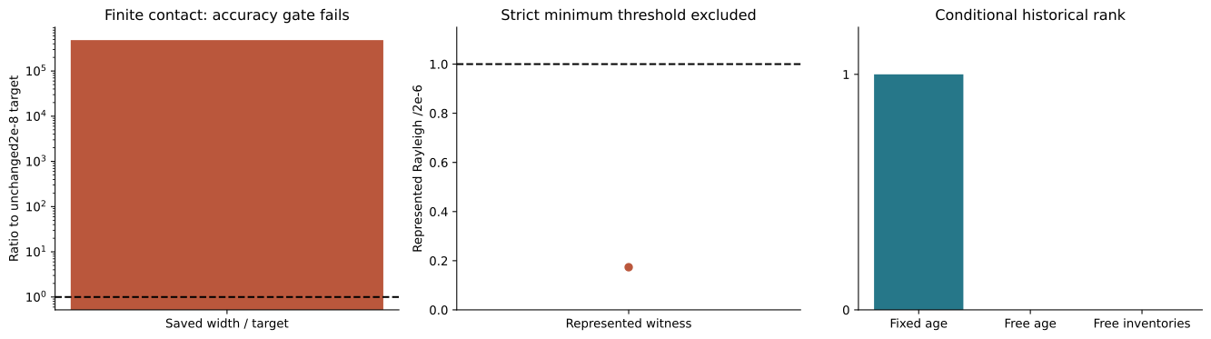
The October 8 continuation adds four independently reviewed results with limited physical scope. Reconstructing all 141 finite screened-contact cells preserves a failed source-width gate: the enclosure width is about 0.00966 against the unchanged target of 0.00000002. One complete 5,778-column Gaussian block has a represented Rayleigh interval below the required minimum threshold; that excludes promotion of this represented block and does not establish a physical negative mode. The Re-only isotope calculation quantifies non-identifiability when chronology or heterogeneous inventories are free. Six planar collision cases reach dimensionless time 120 with walls surviving and rebounding within the finite simulated box; they establish neither complete annihilation into measured pure radiation nor an ordinary-matter history.
A separate analytic diagnostic finds no second static vacuum within |θ| ≤ 0.5 for the selected leading-order canonical QCD axion vacuum potential. It sets no bound on the axion decay constant and excludes neither finite-density nor oscillatory backgrounds. The continuation findings, qualified-result figure, and coverage ledger distinguish these results from method reviews, retained failed attempts and unresolved physical inputs. They do not complete the original research program.