The Metastable Solitude: Could Life Depend on a Rare Persistence Regime?

TL;DR

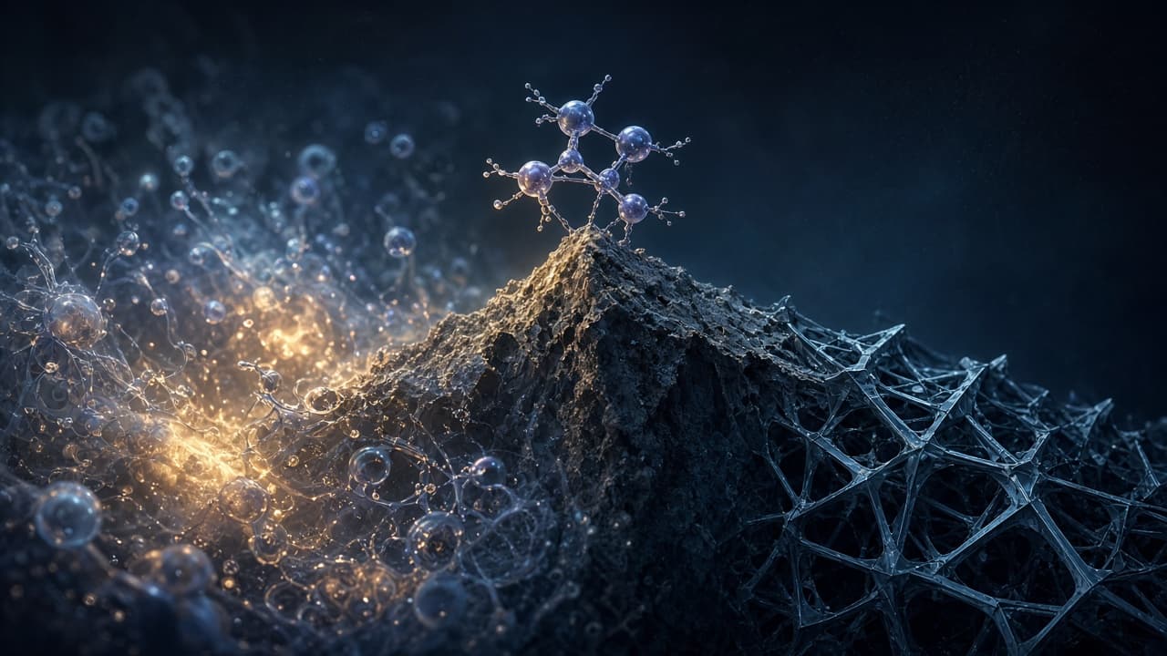
The thought I keep circling is that life may depend less on matter being perfectly stable than on matter being stable for the right amount of time. It needs persistence without permanence: molecules that last, proteins that hold a useful shape, reactions that wait for the right catalyst, and an atmosphere that is reactive without consuming everything at once. Those conditions form a stack of compatible lifetimes. Change enough of them and amino acids might still exist while proteins no longer fold reliably, oxygen no longer participates in a controllable chemistry, or a biochemical network loses the timing that makes it function.

More directly, here is the intuition I am trying to chase:

The central intuition. I am suggesting that something can change in the underlying field description of fundamental particles: the fields whose excitations appear as particles may settle into a different background configuration. Those fields affect one another through specific couplings, so a change in their background values may propagate into dimensionless constants, mass ratios, and the energy barriers inherited by chemistry. Earth may be possible because our region—or our era—currently occupies a rare persistence regime in which elements, compounds, amino acids, proteins, and reaction networks all remain useful on compatible timescales.

This broader claim does not require our universe to occupy a false vacuum. Temperature, pressure, solvent, radiation, catalysis, or another physical phase can reshape a persistence landscape without changing the vacuum at all. The rest of this essay develops changing field and vacuum configurations as one concrete, unusually deep mechanism—not as the premise of the argument.

In that vacuum case study, Earth would exist not only on a habitable planet but during a habitable interval of field history. Two independent histories could surround that interval:

1. Arrival — a higher phase → our phase. A region in a higher-energy configuration might nucleate our lower-energy phase. If the new phase has our constants, that transition could open the chemical window. Regions that have not made the transition—or made it too late—may not have had enough time for complex life.
2. Possible decay — our phase → a lower phase. Our current configuration might itself be a false vacuum above another minimum. A spontaneous bubble of that lower-energy phase could change the local constants and close the chemical window before life or civilization develops.

“Higher” and “lower” here refer only to vacuum energy. They do not mean less or more habitable. A lower phase might be chemically hostile, chemically viable in a different way, or inaccessible for longer than the age of the universe. Neither arrow is inevitable: barriers, tunneling actions, thermal history, and cosmic expansion determine whether a transition occurs at all. In Scenario B, “the necessary conditions have not occurred” can simply mean that no lower-phase bubble has nucleated in our past light cone; it need not mean that ordinary matter has yet to discover a chemical trigger.

The post therefore does not claim that vacuum decay solves the Fermi paradox. It asks whether the broader persistence hypothesis can be made quantitative and, for the vacuum realization, whether the endpoint phases actually change an entire chemical network, spacetime enters and remains in a viable phase for long enough, and that history reduces the number of civilizations in the region we can search even after conditioning on our own existence.

Abstract

Life depends on persistence without permanence. Molecules, macromolecular structures, reaction networks, and planetary reservoirs must remain intact long enough to store information and perform work while remaining changeable enough for selective transformation and renewal. Some are metastable in the strict thermodynamic sense; others are kinetically persistent or maintained as driven disequilibria. This essay asks whether complex life requires a compatible stack of such lifetimes—and whether that stack could be rare across physical environments or cosmic history.

The relevant persistence landscape depends on temperature, solvent, radiation, redox conditions, catalysis, and the dimensionless constants entering the underlying laws. Changes in any of these can alter molecular barriers, reaction rates, conformational lifetimes, and biochemical-network stability. The broad hypothesis is therefore not that life requires one unusually stable substance, but that many coupled processes must remain within mutually compatible ranges.

Changing field or vacuum configurations provide one concrete mechanism for varying the deepest of those conditions. In a specified multi-field theory, distinct minima may realize different dimensionless low-energy constants. As a worked case, I place our observed phase between two candidate minima: a higher-energy phase $A$ that could transition into ours and open a chemically viable interval, and a lower-energy phase $B$ into which ours could decay and close it. These transitions are independent hypotheses; neither is assumed to occur.

That realization works only if it passes three separate gates. First, persistence sensitivity: a specified change of physical background must move a whole reaction and structure network—not merely one favored reaction—outside a defensible viability region. Second, background history: a region must enter a viable regime early enough and remain there continuously for the required emergence time. Third, local relevance: any resulting suppression must survive conditioning on our own existence and operate within the spacetime region we could actually search.

The vacuum realization makes those questions calculable through finite endpoint chemical maps, channel-specific transition dynamics, and observer-conditioned population models. It does not establish that our universe contains the proposed transitions or solve the Fermi question. It turns a broader conjecture about life and metastability into a constrained research program with explicit failure modes.

Introduction: Metastability Before Cosmology

For me, the useful place to begin is not vacuum decay or the Fermi paradox. It is a smaller strangeness: much of what makes life possible is not stable in the absolute sense. It is stable for long enough, and unstable in useful directions.

Metastability is one precise version of that strangeness—the gap between what is thermodynamically preferred and what is kinetically accessible. Imagine a ball resting in a shallow cup halfway down a hillside. The valley below is lower, but the ball cannot reach it until a fluctuation or disturbance carries it over the cup's rim. In thermodynamic language, the cup is a local minimum separated from a lower-energy state by a barrier large compared with the available thermal energy [20]. The depth of the valleys tells us which state equilibrium favors; the barrier and escape path tell us how long the present state can last.

That distinction appears in familiar settings:

• Diamond at ordinary conditions persists even where graphite is favored thermodynamically, because changing the bonded carbon lattice requires a difficult collective rearrangement [21].
• Supercooled water can remain liquid below its equilibrium melting point. Freezing waits for a sufficiently large ice nucleus, so time, temperature, impurities, interfaces, and disturbance all matter [22].
• Oxygen beside fuel stores an obvious chemical possibility without bursting into flame. Ground-state oxygen is a triplet diradical, but its persistence is not explained by spin selection alone: strong bonding makes many initial attacks energetically costly, and reactions with closed-shell molecules can also require access to a different spin surface. Sparks, radicals, metals, light, or enzymes can open faster routes [23]. This is a kinetically persistent mixture, not oxygen sitting in a false vacuum.
• Some proteins inhabit rugged free-energy landscapes with folded basins, intermediates, and misfolded or aggregated traps [24]. A functional structure can be long-lived without being the only—or even the thermodynamically lowest—arrangement available.

“Metastable” therefore does not mean “about to collapse.” A state may last for a fraction of a second or longer than a civilization. Nor is every persistent feature of life a metastable thermodynamic phase. Some are kinetic traps; some, like an oxygen-rich biosphere, are driven disequilibria continuously maintained by flows of energy and matter. I use persistence landscape for this wider family of barriers, pathways, reservoirs, and renewal processes.

A Stack of Lifetimes

The sharper version of the argument is not that a different state must erase amino acids. The building blocks could remain while the relationships that make them useful fail. A protein might no longer hold a functional fold. Oxygen chemistry might become too eager, too sluggish, or too difficult for catalysts to control. Repair might lose its race against damage. A metabolic network might retain every reaction yet lose the relative timing that makes the whole network viable.

Life may therefore require a compatible stack of persistence times:

1. atoms and molecular building blocks must remain available;
2. solvents and planetary reservoirs must occupy useful phases;
3. macromolecules must preserve function without becoming inert;
4. catalysts must cross selected barriers without indiscriminately opening all of them; and
5. repair and replenishment must outrun destructive relaxation.

This formulation is deliberately substrate-neutral. Amino acids, proteins, and oxygen make the idea concrete because they are the chemistry we can test, not because unfamiliar life must use the same materials.

The Version I Am Willing to Defend

Before taking this thought into cosmology, I want to separate it from its most dramatic mechanism. Temperature, pressure, solvent, radiation, and catalysts already change the timing of chemistry without changing the laws beneath it. A material phase change can open one set of pathways and close another. A persistent field background could, in a specified model, reach deeper and alter effective masses or couplings. A vacuum transition is the strangest version of the idea: the fields themselves settle into a different resting configuration, and chemistry inherits the consequences.

The claim I am willing to defend is conditional. Earth-like biochemistry occupies a neighborhood in a high-dimensional map of relative lifetimes. Move far enough in some directions and you leave that neighborhood. What I do not know is whether an allowed change in a fundamental background can move an entire adaptable chemical network across its boundary, whether another cosmic region ever realizes that background, or whether the resulting rarity would still be visible after conditioning on our own existence. I use the vacuum case because it makes the idea sharp enough to fail—not because the universe has given us evidence that this is the mechanism it chose.

From Field Excitations to Interactions

It helps to make “beneath fundamental particles” more concrete. In the weakly-coupled particle picture of quantum field theory, an elementary particle is a quantized excitation of an underlying field. An electron and positron are particle and antiparticle excitations of the same electron field; a muon belongs to another matter field; and a photon is an excitation of the electromagnetic field [25]. A particle is not a bead riding on top of its field, and the fields are not membranes stacked in an extra direction. They coexist throughout the same spacetime. Separating them into lanes is only a way to show which excitation belongs to which field.

Interactions become possible when the theory contains a term coupling those fields. Quantum electrodynamics, for example, contains the two interactions $-eA_\mu\bar\psi_e\gamma^\mu\psi_e$ and $-eA_\mu\bar\psi_\mu\gamma^\mu\psi_\mu$. Together they allow an electron and positron to annihilate and a muon-antimuon pair to emerge, $e^-+e^+\rightarrow\gamma^*\rightarrow\mu^-+\mu^+$, provided the collision has at least the muon-pair threshold energy and satisfies the relevant conservation laws [26]. There is no direct electron–muon–photon vertex; the two QED vertices are essential. The intermediate $\gamma^*$ is an internal contribution to the scattering amplitude—often called a virtual photon—not a separately observable photon following a literal path between the two vertices.

The “bulge” intuition is useful within those limits. The animation uses the real projection of a Morlet-wavelet profile, $\operatorname{Re}\psi_M(u)\propto e^{-u^2/2}[\cos(\omega_0u-\omega t)-e^{-\omega_0^2/2}]$, as a one-dimensional visual proxy for a localized state. The translated, Gaussian-windowed carrier is an animation convention, not a time-evolved Morlet solution of a particle field equation. That signal is still a schematic amplitude—not a measurement of a fermion field's literal height. What changes lanes is the amplitude assigned to allowed field configurations, not a physical sheet pushing through a neighboring sheet.

Field-interaction primer. Follow Morlet wave packets through a schematic account of an allowed QED amplitude, then into two deliberately different toy continuations. In the local route, an outgoing product later deposits energy in a nearby target and may push its state across a pre-existing barrier while $U(q)$ remains fixed. In the separate background counterfactual, the potential itself changes and the persistence time changes with it. The second route is not caused by this scattering, and neither route is a prediction for a particular material. The separated field lanes are bookkeeping, not a literal microscopic movie.

Why a Background Field Is Different

One scattering event changes a state, not a law. It changes the particles involved, but it does not rewrite the fine-structure constant, move the surrounding region into another vacuum, or alter chemistry's rules everywhere. Local reactions can certainly trigger a phase change when a system is already poised near a barrier. A trigger, however, is different from changing the landscape that contains the barrier.

Many excitations can nevertheless matter collectively. A thermal or dense bath can reshape an effective potential or a medium's response, and one energetic event can seed a transition whose lower state was already available [19]. Neither is the same as a few random particles rewriting the fundamental Lagrangian.

A systematic downstream shift needs a persistent background field value, coherent state, medium, or phase that many interactions inherit. The familiar Higgs background helps set particle masses. More speculatively, a background scalar coupled to gauge, Yukawa, or strong-sector operators could change effective dimensionless inputs across a region [4, 11]. In a physical model, the intuition that fields “harmonize” therefore has to become specific through coupling functions stated by the theory. Those changes would propagate: field background → constants and mass ratios → atomic and molecular energy scales → reaction barriers and conformational landscapes → persistence times. Because rates can depend exponentially on barrier height [5], a modest underlying shift may have a large downstream effect—but whether it does is a calculation, not an assumption.

Interactive primer. Explore a background-to-chemistry path through four familiar persistence analogies. The controls use normalized, illustrative responses rather than predicting alternate diamond, water, oxygen, or protein chemistry. They show the causal structure a real model would need to calculate.

The rest of the essay investigates changing field or vacuum configurations as one candidate source of the deepest variation in this stack. A vacuum, in this context, is a resting configuration of fields—not merely empty space. Different minima can yield different low-energy physics only when explicit couplings make them do so. The vacuum picture below is a worked case of the broader persistence hypothesis, not its prerequisite.

1. From Persistent Chemistry to Cosmic Rarity

The grand temptation is to leap from fragile chemistry to the silence of the sky. I do not want to smuggle that leap in. The Fermi question begins with a mismatch: a very large cosmos appears to offer many opportunities for technological life, while our searches have produced no widely accepted evidence of it [1]. But the input probabilities are uncertain enough that this mismatch should not be treated as a theorem. Sandberg, Drexler, and Ord showed how broad uncertainties in the usual Drake factors can dissolve much of the apparent paradox [2]. Any new proposal should sharpen a conditional probability, not simply add another dramatic filter.

The broad hypothesis is that life requires many persistence and turnover times to remain mutually compatible. The vacuum realization tested here asks whether three more specific links can hold at once:

1. A joint field landscape contains several minima, and cosmological dynamics populate regions or epochs with different dimensionless constants.
2. Our observed phase permits Earth-like complex chemistry, while at least one specified endpoint phase lies outside a quantitative chemical viability region.
3. Regions enter our phase late, leave it early, or remain too isolated for many civilizations to overlap inside our searchable neighborhood—even after conditioning on the fact that our own lineage had time to emerge.

Anthropic work has often emphasized the wider boundaries imposed by nuclear stability and stellar evolution [14]. The claim tested here is that an Earth-like chemical network could occupy a stricter region inside those boundaries. That nesting is a hypothesis, not an established hierarchy.

The scope matters. The persistence hypothesis is substrate-neutral, but the quantitative case study is necessarily narrower: I use “chemical viability” to mean viability for complex Earth-like biochemistry, not impossibility for every conceivable substrate or form of life. I distinguish two directions through the landscape. In Scenario A, a higher-energy parent phase nucleates regions of our phase; the question is when and where the chemical window opens. In Scenario B, our phase nucleates a still-lower daughter phase; the question is how long the window remains open. Each arrow needs its own potential barrier, bounce solution, and endpoint chemistry. Either arrow may be absent.

Transition direction is separate from spacetime geometry. A first-order transition can produce expanding bubbles and temporarily coexisting regions. An early symmetry-breaking event can instead leave a persistent domain mosaic, and a sufficiently completed transition can look like a change between broad cosmic epochs. Those histories have different observations and different relevance to nearby life.

The interesting question, then, is not whether chemistry depends on its physical background—from solvent and radiation to the constants of the underlying theory—but whether a narrow persistence regime survives every available escape hatch: adaptation, screening, vacuum geometry, and the fact that we are already here to ask.

2. One Deep Mechanism: What Varies Between Field Phases?

2.1. A Minimal Effective Description

For readable notation, begin with one canonically normalized effective coordinate $\phi$ coupled to gravity and Standard Model sectors:

For illustration, the electromagnetic and fermion-mass terms can be written as

Only dimensionless combinations are observable. A useful coordinate vector is

A vacuum expectation value is the average value a field takes in a specified quantum state. A minimum of the effective potential is a candidate phase; it is metastable when it is locally trapped behind a barrier but has a nonzero decay amplitude to a lower-energy configuration [6]. In that precise sense, the suggested “harmonizing” of several fields is a joint background location in field space, not a collision among a few particle excitations. Whether that location changes particle masses or interactions then follows from the coupling functions in the specified theory—it is not guaranteed merely by the existence of another minimum.

The coordinate $\phi$ can represent a collective path through a genuinely multidimensional field configuration $\boldsymbol{\phi}=(\phi_1,\ldots,\phi_n)$. In a full model, the fields need not change in lockstep: a multi-field bounce can follow a curved trajectory through field space, and its coupled dynamics must be solved rather than inferred from this one-dimensional sketch [17].

The potential $V(\boldsymbol{\phi})$ may possess several minima [3, 17]. The clarified toy landscape uses three:

$A$ is a possible higher-energy parent, “us” is the phase whose constants we observe, and $B$ is a possible lower-energy daughter. The arrows $A\rightarrow\mathrm{us}$ and $\mathrm{us}\rightarrow B$ are separate candidate transitions. This ordering says nothing by itself about chemistry. The claim that $A$ or $B$ is chemically nonviable must be established independently by Gate I.

Multiple minima also do not guarantee that multiple phases are populated inside our observable universe. Quantum tunneling, finite-temperature phase evolution, and causal selection of different minima are distinct mechanisms. The bubble models below focus on first-order tunneling; the domain discussion treats early vacuum selection separately [6, 7, 18, 19]. There is no generic rule that every higher phase quickly converges to the next lower one.

Figure 1. Schematic effective path through a multi-field landscape. Scenario A asks whether a higher-energy parent can nucleate our observed phase. Scenario B asks whether our phase can nucleate a lower-energy daughter. The arrows and chemical status of either endpoint are model hypotheses; vacuum-energy depth does not determine habitability.

2.2. Local Derivatives Are Not Finite Vacuum Jumps

Two quantities must remain distinct. Experiments performed in our vacuum probe local scalar derivatives,

Chemistry in two different minima depends instead on the finite jump

For the three-phase sketch, the two signed endpoint changes are

The labels “in” and “out” identify the proposed histories, not motion through every intermediate low-energy theory. Chemistry may respond very differently to the two endpoint comparisons.

There is no model-independent inequality that turns a fifth-force bound on $d_i^{\mathrm{us}}$ into a bound on $\Delta_i^{\mathrm{vac}}$. A coupling function can be flat near our minimum yet differ substantially at another one; conversely, a large local slope can be hidden only if the field is massive, screened, or otherwise prevented from sourcing an observable force. A linear expansion across the full excursion is a useful benchmark, but it is an extra assumption rather than a general fact.

This distinction prevents a common shortcut: precision experiments near our minimum and chemical differences between minima constrain different parts of a candidate model. Measurements in our phase do not determine the local derivatives near $A$ or $B$, either finite jump, or either bounce action. A complete EFT must calculate each quantity it uses.

3. Gate I: Reaction-Network Sensitivity

3.1. From One Barrier to a Matrix of Rates

For a reaction $j$, transition-state theory gives the schematic rate

where $\kappa_j$ is a transmission factor and $\Delta G_j^\ddagger$ is the activation free energy [5]. Changing the constants can alter the barrier, the prefactor, solvent properties, and the range of viable temperatures. The full linear response is therefore

Here $\Delta G_j^\ddagger$ is written per reacting entity. If it is instead a molar free energy, the same Eyring expression uses $RT$ in place of $k_BT$. Keeping those conventions separate matters when comparing a barrier estimate with an activation-energy table. At fixed barrier and temperature, increasing the rate prefactor shortens the mean waiting time; it does not lengthen it.

If temperature and the prefactor are held fixed for a local estimate, the barrier contribution is

This is the honest content of the familiar exponential amplification. A small change in a dimensionless constant can produce a large change in a log rate when the absolute barrier derivative is large compared with $k_BT$. It does not follow that one order-unity rate change kills a metabolism. Biological networks contain feedback, redundancy, catalytic adaptation, and environmental degrees of freedom.

It is tempting to define

so that $S_{ji}^{(\mathrm{barrier})}\approx-\Theta_jK_{ji}$. But a huge fractional $K_{ji}$ caused by a cancellation inside a small barrier is not automatically a huge physical effect: the product $\Theta_jK_{ji}$ depends on the absolute derivative of the barrier. The quantity to calculate is $S$, not an isolated fractional coefficient.

For the interactive one-direction projection below, hold the prefactor and temperature fixed and write $\mathcal{A}=\Delta G^\ddagger/k_BT$. The kinetic exponent and exact local rate ratio are then

This scalar projection is useful for intuition; $S$ is the local object a real network calculation must estimate before attempting finite changes.

Figure 2. Deterministic reaction-rate sensitivity instrument. The paired barriers and seeded thermal opportunities illustrate the exact rate ratio within the displayed one-direction model. They do not depict a literal molecule or establish network-level sterility.

3.2. Finite Jumps Need a Nonlinear Map

The Jacobian $S$ is a tangent-space description. Applying $S\Delta^{\mathrm{vac}}$ to an unrestricted jump between distant minima would silently assume that the chemistry remains linear along the whole excursion. For a path $\mathbf{C}(\lambda)$ connecting the two endpoint theories, the finite log-rate difference is instead

Equivalently, one can calculate the rates independently in both vacua and take their log ratio. The interpolation is bookkeeping, not an assertion that the universe physically traverses every intermediate theory; it must vary masses, binding energies, solvents, and environmental optima consistently. Only for a small jump in a genuinely linear regime does this reduce to $\Delta\ln\mathbf{k}^{\mathrm{vac}}\approx S_{\mathrm{us}}\Delta^{\mathrm{vac}}$.

3.3. A Network-Level Chemical Viability Window

Let $W$ encode which combinations of log rates a candidate biochemical network can tolerate after allowing specified environmental and regulatory adjustments. A finite Chemical Viability Window (CVW) can then be defined by

Near our vacuum, along a unit direction $\mathbf{u}$ in constant space, its linearized half-width is

This width is inversely proportional to sensitivity. The Arrhenius exponential does not make the interval exponentially narrow. A high-dimensional viable volume may still become very small if several independent, strongly constrained rate combinations must be satisfied simultaneously, but even the local conclusion requires the spectrum of $W S_{\mathrm{us}}$, not rhetoric about one typical activation energy. Distant vacua require the finite map above.

Gate I is therefore concrete, and directional:

For Scenario A, calculate whether $\mathbf{C}_A$ lies outside the relevant chemical viability region while $\mathbf{C}_{\mathrm{us}}$ lies inside it. For Scenario B, repeat the endpoint calculation for $\mathbf{C}_{\mathrm{us}}$ and $\mathbf{C}_B$. Vacuum-energy ordering answers neither question, and a model using only one arrow need not make both remote endpoints nonviable.

Figure 3. Log-log map of the one-direction necessary condition $\eta_{\mathrm{kin}}\ge\eta_{\mathrm{crit}}$. Crossing its boundary means the chosen rate perturbation is kinetically consequential, not that a biochemical network is necessarily nonviable.

The gate is deliberately difficult. Existing calculations of atomic and molecular transition frequencies show that some observables have enhanced sensitivity to varying constants, but that is not yet a calculation of activation-free-energy derivatives for a viable metabolic network. Until such a matrix exists, a “chemically nonviable endpoint phase” remains a hypothesis.

4. Gate II: Opening and Preserving the Habitable Phase

4.1. Two Directions, One Residence Window

Scenario A is an entry problem. Regions begin in a higher-energy phase $A$; our phase nucleates within it. The proposed chemical window opens only after the new phase arrives, and complex life requires enough subsequent time for structure, planets, and biology. Scenario B is an exit problem. A region already in our phase remains chemically permissive only until a $B$ bubble reaches its worldline.

Writing $A\rightarrow\mathrm{us}\rightarrow B$ organizes those possibilities; it does not assert that both arrows exist or that our region completed the first and now awaits the second. The shared quantity is the probability of uninterrupted residence in our phase along a candidate worldline $\gamma$ for a biological interval $\tau_{\mathrm{bio}}$:

This condition is stricter than occupying our phase at one instant. It rejects regions reached too late by Scenario A and regions exited too early by Scenario B. It also assumes that the transition and its released energy leave or rebuild the astrophysical conditions required for life—another calculation a complete model cannot skip.

4.2. First-Order Conversion in Either Direction

For either proposed arrow $q\in\{A\rightarrow\mathrm{us}, \mathrm{us}\rightarrow B\}$, a first-order transition can be modeled by bubbles nucleating at a rate per physical four-volume

where $B$ is the channel-specific bounce-action difference and $A_{\mathrm{vac}}$ contains the fluctuation prefactor [6, 17]. Once a supercritical bubble forms, its subsequent growth depends on the potential, wall dynamics, gravity, and surrounding spacetime. The result is a stochastic conversion process, not a field value smoothly sliding over the barrier or a static checkerboard. The two arrows need not have remotely similar rates. At zero temperature, this decay does not wait for matter to discover a chemical trigger; “conditions not yet met” can simply mean that the quantum nucleation rate is extraordinarily small. Thermal transitions or environmental catalysis are separate, model-dependent possibilities [19].

For a homogeneous Friedmann-Robertson-Walker background, the expected nucleated four-volume capable of reaching an event at time $t$ can be written schematically as [7]

where $v_w$ is the wall speed. The probability that the parent phase still occupies that event is

For Scenario A, $1-P_{\mathrm{meta}}$ is a local conversion probability, but a life model also needs the age and post-transition history of the new region. For Scenario B, $P_{\mathrm{meta}}$ is the probability that our phase has survived at the event.

In flat spacetime, with constant $\Gamma$ and nucleation beginning at $t=0$, this reduces to

For luminal walls ($v_w=1$), this is the familiar $\pi\Gamma t^4/3$ result. That fourth power is important. A decay rate per four-volume does not generically produce the constant-hazard form $e^{-t/\tau}$. Such an exponential can still be explored as a phenomenological toy, but it should not be mistaken for the vacuum-decay calculation.

Figure 4. The same schematic bubble geometry can play two causal roles. In Scenario A, bubbles of our phase expand through a higher-energy parent and open the chemical window. In Scenario B, lower-energy daughter bubbles expand through our phase and may close it. The colors identify phases, not habitability inferred from energy. The picture suppresses wall dynamics, collisions, gravity, and the physics inside either daughter phase.

4.3. Scenario B: Survival After Entry

This subsection isolates Scenario B and assumes entry into our phase has already occurred. Let $\rho_{\mathrm{civ}}(t)$ be a baseline density of civilization-emergence events after accounting for star and planet formation. The normalized overlap between that history and survival of our phase is

This ratio is dimensionless and equals one in the stable-vacuum limit. If the emergence history is idealized as a delta function at $\tau_{\mathrm{civ}}$,

For comparison, a phenomenological constant-hazard model with $P_{\mathrm{meta}}=e^{-t/\tau_{\mathrm{vac}}}$ gives

Equal timescales then yield $F_{\mathrm{surv}}=e^{-1}\approx0.37$: only a factor of $e\approx2.7$ attenuation, not an explanation of $N\ll1$ by itself. Strong suppression requires a much larger survival exponent, and our own existence makes that choice an anthropically selected outcome.

Figure 5. Scenario B only: animated emergence–survival overlap after a region has entered our phase. The figure compares a constant-hazard kernel with the $t^4$ scaling of the flat-spacetime bubble toy. Its shared time-scale control marks the point where either kernel reaches $e^{-1}$, not a common mean lifetime; the physically motivated curve must still be computed from $I(t)$ for a specified cosmology and exit history.

For the full two-sided model, the corresponding phase-history factor is

Here $\rho_{\mathrm{civ}}^{(0)}$ is only a reference emergence history. If $A$ or $B$ can support a different form of life, each phase needs its own structure, stellar, chemical, and emergence model rather than one baseline multiplied by a survival probability.

Gate II is satisfied only when specified entry and/or exit histories produce a small $F_{\mathrm{phase}}$ while remaining compatible with the age and observed history of our own region.

4.4. Transition Direction Is Not Spacetime Geometry

Scenario A and Scenario B name directions through a potential. “Domain,” “bubble,” and “epoch” describe how the phases are distributed in spacetime. An incomplete first-order transition can leave coexisting regions; a completed transition can separate approximate cosmic epochs. An early symmetry-breaking or vacuum-selection event can instead leave regions that chose different minima before galaxies formed. Its critical inputs are the population of each vacuum, the comoving domain-size distribution, inflationary dilution, and the fate of the walls [18].

Persistent domain walls carry stress-energy and are strongly constrained by cosmology [15, 16]. Biased vacua may cause walls to collapse; inflation may push other domains beyond our horizon. Either escape can make the domains difficult to observe, but it can also remove their ability to explain silence inside our search volume. Ancient selection, entry bubbles, and possible late decay should therefore be tested as distinct occupancy histories, not combined into one “percolation” picture. Even when a lower-energy phase is available, a transition can be so suppressed that no relevant bubble forms; local worldline conversion, global volume conversion, and percolation are not interchangeable claims [7].

5. Gate III: From Global Rarity to Local Silence

5.1. The Observer-Conditioning Problem

A small global viable fraction is not yet a Fermi filter. We know that at least one viable region survived long enough to produce us. The relevant comparison is the number of peers expected conditional on that fact:

Here $O_{\mathrm{us}}$ includes our chemical viability, entry time, and long uninterrupted residence in our phase; $N_{\mathrm{peers}}$ counts civilizations in a defined searchable region. If that entire region shares our phase history, conditioning on $O_{\mathrm{us}}$ can make its neighbors much more likely to be viable than a random spacetime point. Multiplying an ordinary Drake estimate by the global $F_{\mathrm{phase}}$ would then double-count our surprise.

A stationary ancient-domain picture has a simple necessary scale hierarchy:

Domains must be large enough to host stable biospheres but small enough that our search volume samples more than the one selected by our existence. Entry and exit bubbles do not have a fixed $L_{\mathrm{domain}}$, so their analogous calculation must use the joint phase histories of our worldline and the candidate worldlines. Conditioning on our presence inside an old Scenario A bubble favors nearby locations that share its entry history. Conditioning on no Scenario B bubble having reached us likewise favors nearby worldlines with correlated survival histories.

A schematic peer count is

This is where cosmology actually meets the Fermi question. Gate III is passed only if a specified phase-history model drives $F_{\mathrm{obs}}\ll1$, not merely if a random point in a much larger universe is unlikely to support life.

Figure 6. Observer-conditioned accounting on a shared logarithmic scale. The interactive uses the Scenario B emergence–survival slice from Figure 5, then restores an illustrative shared-history dependence between our known viable region and the region we can search. A full two-sided model would replace that slice with $F_{\mathrm{phase}}$. The interpolation is illustrative; a physical value must come from the conditional integral above rather than an independent Drake factor.

6. Constraints and Falsifiers

The framework has three distinct constraint classes. Keeping them separate makes the hypothesis harder to rescue by moving one parameter.

6.1. Chemical Constraints

The first empirical target is the local matrix $S$, followed by the nonlinear finite rate map between specified endpoint theories. The calculation should use dimensionless constants, activation free energies, solvent and catalytic effects, and a network-level viability criterion. A result in which realistic adaptation keeps $\|W\Delta\ln\mathbf{k}^{\mathrm{vac}}\|$ small across plausible vacuum jumps would close the chemical gate.

Conversely, finding a few spectroscopic transitions with large sensitivity is not enough. The claim needs large, differently directed changes in reactions whose relative rates cannot all be restored by temperature, regulation, or evolution.

6.2. Local Scalar Constraints

The cited precision-spectroscopy analysis finds no robust cosmological drift in $\alpha$ at approximately the part-per-million level along well-controlled quasar sightlines [8]. Methanol systems constrain changes in $\mu=m_p/m_e$ at roughly the $10^{-7}$ level for particular absorbers [9]. These are powerful measurements of sampled environments inside our past light cone. They are not universal bounds on an unsampled upstream or downstream phase.

Tests of the Weak Equivalence Principle are even more stringent: the final MICROSCOPE result found no violation at the few-parts-in-$10^{15}$ level in the Eötvös ratio [10]. Translating that result into a bound on one scalar coupling requires its mass, range, and composition-dependent dilaton charges [11]. A single universal $\beta_{\max}$ hides that model dependence.

Within the restricted benchmark of a linear, unscreened coupling across a field excursion,

One effective chemical direction would then need to satisfy the linear-regime gate

This is a necessary condition only for that benchmark and only while an endpoint is close enough for an expansion around our phase to remain controlled. A distant $A\rightarrow\mathrm{us}$ comparison generally requires the full coupling functions or an expansion around $A$. The benchmark replaces the earlier universal product $K_{\mathrm{eff}}\beta_{\max}$, which conflated local force bounds with finite inter-vacuum differences.

Chameleon and symmetron mechanisms can suppress local field profiles in dense environments [12, 13]. They do not simply “increase the allowed coupling,” and a molecular cloud is not generically screened. Any screened realization must solve for the scalar profile in the laboratory, Solar System, absorber, and intergalactic environments used in the comparison.

6.3. Bubble, Wall, and Sky Constraints

Scenario A may leave signatures from bubble collisions, curvature, reheating, or altered perturbations, depending on when entry occurred and whether later inflation erased them. In Scenario B, an intersecting lower-energy daughter bubble could be catastrophic rather than a quiet region with unfamiliar spectral lines. The absence of such an event constrains the integrated exit history in our past light cone. In an ancient-domain model, surviving walls affect the cosmic expansion and generate CMB temperature and polarization power; modern analyses place strong limits on stable wall networks [15, 16]. The line-like Gott–Kaiser–Stebbins discontinuity belongs specifically to cosmic strings and should not be used as a generic wall prediction.

Useful observational tests include correlated, non-Gaussian changes across multiple transitions with different sensitivity coefficients; consistency between $\alpha$, $\mu$, and clock data; and CMB or lensing constraints tied to an explicitly calculated wall stress-energy. A synthetic patchwork is useful for learning what spatial coherence would mean, but it is not itself a predicted sky.

Figure 7. Seeded synthetic domains sampled by a finite spectroscopic survey. The animation accumulates fixed sightlines and tests a known spatial template against noise; it visualizes discriminating power, not discovery significance. It is neither a CMB realization nor evidence for domains.

The proposal would be substantially weakened or falsified within a specified model if any of the following occurred:

• quantum chemistry and network adaptation kept candidate biochemical systems viable across every allowed $\Delta^{\mathrm{vac}}$;
• a complete scalar model could not satisfy local force, clock, and spectroscopic constraints simultaneously;
• the required entry or exit history contradicted the age and uninterrupted residence of our region;
• the domain correlation length lay entirely beyond the search volume after conditioning on us;
• walls or spatial variations required for local suppression exceeded CMB, large-scale-structure, or spectroscopy bounds.

6.4. Where This Story Could Break

The first danger is chemical robustness. Life does not inherit a frozen list of rate constants. It changes catalysts, concentrations, regulation, temperature, solvent activity, and sometimes the pathway itself. Life is, in other words, very good at routing around trouble. A network may remain viable even when each individual reaction changes substantially. That is why Gate I asks for an optimized network-level failure, not one molecule with a spectacular sensitivity coefficient.

The second is substrate freedom. I keep reaching for proteins, water, and oxygen because they are the chemistry we can interrogate, not because the universe owes life our recipe. Closing their window would not prove that all organized, evolving matter is impossible. A broader claim needs either a substrate-independent requirement—reliable information storage and selective turnover, for example—or separate models for other candidate substrates.

The third problem is that drawing extra valleys is cheap. A theory can contain additional minima without ever placing one in our observable history, and those minima can leave the low-energy constants almost unchanged. Multiple vacua, finite jumps in constants, chemically consequential endpoint differences, and an astrophysically relevant transition history are four separate propositions. The existence of the first does not buy the other three.

Finally, the quiet sky may not need any of this. Uncertain biogenesis rates, evolutionary bottlenecks, short technological lifetimes, limited search coverage, or ordinary astrophysical selection can each reduce the expected signal [2]. This persistence hypothesis earns explanatory work only if it improves a joint population model after those alternatives and our own selection effect are included. Otherwise it remains what it started as: an interesting way to map chemical contingency, not an explanation for an empty sky.

7. What Would Turn the Idea Into a Model?

If this is more than a suggestive picture, it has to survive four calculations.

1. A persistence sensitivity map. First map reaction, folding, degradation, and renewal times across environmental background parameters. Then compute $S_{ji}$ for a curated set of catalytic and non-catalytic reactions, extend it to finite endpoint differences while varying dimensionless constants consistently, and propagate those changes through a robust network model.
2. A benchmark multi-field EFT. Specify the candidate minima of $V(\boldsymbol{\phi})$, all relevant coupling functions, the masses and constants in each phase, and any screening profile. For every retained arrow, calculate its finite chemical map, bounce solution, wall dynamics, and transition rate rather than identifying these quantities with one another.
3. A phase-residence calculation. Derive the distribution of entry times, exit times, and uninterrupted residence durations in the chosen cosmology; include what the transitions do to pre-existing or newly forming stars and planets, then convolve that history with realistic emergence times.
4. An observer-conditioned population model. Infer $N_{\mathrm{peers}}$ jointly with our existence and survey volume, including the domain correlation structure. This determines whether global scarcity becomes local solitude.

Each calculation can fail independently. I think that is a virtue. The idea should earn credibility by surviving gates that are actually able to kill it.

8. Conclusion

I began with a suspicion about timing: life may depend on a compatible hierarchy of persistence times rather than on a single privileged substance. The building blocks can survive while protein folds, oxygen chemistry, catalytic selectivity, repair, or network timing becomes unworkable. A life-permitting regime could therefore be restricted across environments and epochs even when many of its ingredients remain present.

Following that suspicion all the way down leads to vacuum history as one candidate mechanism for varying the deepest layer of the hierarchy. In the worked realization, our phase is the empirically known chemically permissive middle state in a toy three-minimum landscape. Scenario A asks whether regions enter it early and broadly enough. Scenario B asks whether they remain in it long enough. Neither arrow is guaranteed, and a lower valley in vacuum energy does not tell us whether its chemistry is a garden, a desert, or something for which we have no word.

The three gates are there to keep the interesting parts of the story from sliding into one another. The chemical gate is a nonlinear finite rate map applied independently to specified endpoints, with the reaction-network sensitivity matrix as its local diagnostic. The cosmological gate is the entry–residence–exit history built from channel-specific nucleation dynamics. The Fermi gate is observer-conditioned and local, not a global spacetime fraction. Local fifth-force measurements, finite vacuum jumps, and domain-wall constraints then occupy distinct roles rather than one universal “constraint budget.”

Nothing presented here establishes that our universe realizes either transition or that a different persistence regime would be lifeless. The more modest conclusion is useful enough. What keeps pulling me back to the idea is that the fit among many chemical lifetimes is a physical condition we can map rather than a vague synonym for “habitability.” Vacuum transitions are one way that condition could vary, and probably the hardest one to make work. Cosmic solitude would follow only if the persistence tests, phase-entry or phase-exit history, and observer-conditioned locality all point in the same direction.

References

[1] M. H. Hart, “An Explanation for the Absence of Extraterrestrials on Earth,” Quarterly Journal of the Royal Astronomical Society 16, 128–135 (1975).

[2] A. Sandberg, E. Drexler, and T. Ord, “Dissolving the Fermi Paradox,” arXiv:1806.02404 (2018).

[3] R. Bousso and J. Polchinski, “Quantization of Four-Form Fluxes and Dynamical Neutralization of the Cosmological Constant,” Journal of High Energy Physics 2000(06), 006 (2000). doi:10.1088/1126-6708/2000/06/006.

[4] J.-P. Uzan, “Varying Constants, Gravitation and Cosmology,” Living Reviews in Relativity 14, 2 (2011). doi:10.12942/lrr-2011-2.

[5] H. Eyring, “The Activated Complex in Chemical Reactions,” The Journal of Chemical Physics 3, 107–115 (1935). doi:10.1063/1.1749604.

[6] S. Coleman and F. De Luccia, “Gravitational Effects on and of Vacuum Decay,” Physical Review D 21, 3305–3315 (1980). doi:10.1103/PhysRevD.21.3305.

[7] A. H. Guth and E. J. Weinberg, “Could the Universe Have Recovered from a Slow First-Order Phase Transition?” Nuclear Physics B 212, 321–364 (1983). doi:10.1016/0550-3213(83)90307-3.

[8] M. T. Murphy et al., “Fundamental Physics with ESPRESSO: Precise Limit on Variations in the Fine-Structure Constant Towards the Bright Quasar HE 0515−4414,” Astronomy & Astrophysics 658, A123 (2022). doi:10.1051/0004-6361/202142257.

[9] J. Bagdonaite et al., “A Stringent Limit on a Drifting Proton-to-Electron Mass Ratio from Alcohol in the Early Universe,” Science 339, 46–48 (2013). doi:10.1126/science.1224898.

[10] P. Touboul et al., “MICROSCOPE Mission: Final Results of the Test of the Equivalence Principle,” Physical Review Letters 129, 121102 (2022). doi:10.1103/PhysRevLett.129.121102.

[11] T. Damour and J. F. Donoghue, “Equivalence Principle Violations and Couplings of a Light Dilaton,” Physical Review D 82, 084033 (2010). doi:10.1103/PhysRevD.82.084033.

[12] J. Khoury and A. Weltman, “Chameleon Fields: Awaiting Surprises for Tests of Gravity in Space,” Physical Review Letters 93, 171104 (2004). doi:10.1103/PhysRevLett.93.171104.

[13] K. Hinterbichler and J. Khoury, “Screening Long-Range Forces Through Local Symmetry Restoration,” Physical Review Letters 104, 231301 (2010). doi:10.1103/PhysRevLett.104.231301.

[14] C. J. Hogan, “Why the Universe Is Just So,” Reviews of Modern Physics 72, 1149–1161 (2000). doi:10.1103/RevModPhys.72.1149.

[15] L. Sousa and P. P. Avelino, “Cosmic Microwave Background Anisotropies Generated by Domain Wall Networks,” Physical Review D 92, 083520 (2015). doi:10.1103/PhysRevD.92.083520.

[16] A. Lazanu, C. J. A. P. Martins, and E. P. S. Shellard, “Contribution of Domain Wall Networks to the CMB Power Spectrum,” Physics Letters B 747, 426–432 (2015). doi:10.1016/j.physletb.2015.06.034.

[17] V. Balasubramanian, B. Czech, K. Larjo, and T. S. Levi, “Vacuum Decay in Multidimensional Field Landscapes: Thin, Thick and Intersecting Walls,” Physical Review D 84, 025019 (2011). doi:10.1103/PhysRevD.84.025019.

[18] T. W. B. Kibble, “Topology of Cosmic Domains and Strings,” Journal of Physics A: Mathematical and General 9, 1387–1398 (1976). doi:10.1088/0305-4470/9/8/029.

[19] A. D. Linde, “Decay of the False Vacuum at Finite Temperature,” Nuclear Physics B 216, 421–445 (1983). doi:10.1016/0550-3213(83)90293-6.

[20] IUPAC, “Metastable State,” Compendium of Chemical Terminology (the Gold Book), 5th ed. doi:10.1351/goldbook.M03871.

[21] F. P. Bundy, W. A. Bassett, M. S. Weathers, R. J. Hemley, H. U. Mao, and A. F. Goncharov, “The Pressure-Temperature Phase and Transformation Diagram for Carbon; Updated through 1994,” Carbon 34, 141–153 (1996). doi:10.1016/0008-6223(96)00170-4.

[22] T. Koop, B. Luo, A. Tsias, and T. Peter, “Water Activity as the Determinant for Homogeneous Ice Nucleation in Aqueous Solutions,” Nature 406, 611–614 (2000). doi:10.1038/35020537.

[23] W. T. Borden, R. Hoffmann, T. Stuyver, and B. Chen, “Dioxygen: What Makes This Triplet Diradical Kinetically Persistent?” Journal of the American Chemical Society 139, 9010–9018 (2017). doi:10.1021/jacs.7b04232.

[24] J. N. Onuchic, Z. Luthey-Schulten, and P. G. Wolynes, “Theory of Protein Folding: The Energy Landscape Perspective,” Annual Review of Physical Chemistry 48, 545–600 (1997). doi:10.1146/annurev.physchem.48.1.545.

[25] F. Quevedo and A. Schachner, “Cambridge Lectures on the Standard Model,” arXiv:2409.09211 (2024). doi:10.48550/arXiv.2409.09211.

[26] S. Navas et al. (Particle Data Group), “Review of Particle Physics,” Physical Review D 110, 030001 (2024), Sec. 51, “Cross-Section Formulae for Specific Processes.” doi:10.1103/PhysRevD.110.030001.